In the chapters that follow, I show you the essentials of Python. I start from the absolute basics of what makes a Python program and move through Python’s built-in data types and control structures, as well as defining functions and using modules. The last chapter of this part moves on to show you how to write standalone Python programs, manipulate files, handle errors, and use classes.
4. The absolute basics
This chapter covers
Indenting and block structuring
Differentiating comments
Assigning variables
Optional type hints
Evaluating expressions
Using common data types
Getting user input
Using correct Pythonic style
This chapter describes the absolute basics in Python: how to use assignments and expressions, how to use numbers and strings, how to indicate comments in code, and so forth. It starts with a discussion of how Python block structures its code, which differs from every other major language.
4.1 Indentation and block structuring
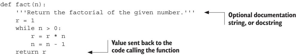
Python differs from most other programming languages because it uses whitespace and indentation to determine block structure (that is, to determine what constitutes the body of a loop, the else clause of a conditional, and so on). Most languages use braces of some sort to do this. The following is C code that calculates the factorial of 9, leaving the result in the variable r:
/* This is C code */int n, r;n =9;r =1;while(n >0){ r *= n; n--;}
The braces delimit the body of the while loop, the code that is executed with each repetition of the loop. The code is usually indented more or less as shown, to make clear what’s going on, but it could also be written as follows:
/* And this is C code with arbitrary indentation */int n, r; n =9; r =1;while(n >0){r *= n;n--;}
The code still would execute correctly, even though it’s rather difficult to read. The Python equivalent is
# This is Python code.n =9r =1while n >0: r = r * n # Python also supports C-style r *= n. n = n -1# Python also supports n –= 1.
Python doesn’t use braces to indicate code structure; instead, the indentation itself is used. The last two lines of the previous code are the body of the while loop because they come immediately after the while statement and are indented one level further than the while statement. If those lines weren’t indented, they wouldn’t be part of the body of the while.
Note that while it’s more explicit and clearer to say r = r * n, it’s also possible and good Pythonic style to use the shorter r *= n form—both are fine in Python.
Using indentation to structure code rather than braces may take some getting used to, but there are significant benefits:
It’s impossible to have missing or extra braces. You never need to hunt through your code for the brace near the bottom that matches the one a few lines from the top.
The visual structure of the code reflects its real structure, which makes it easy to grasp the skeleton of the code just by looking at it.
Python coding styles are mostly uniform. In other words, you’re unlikely to go crazy from dealing with someone’s idea of aesthetically pleasing code. Everyone’s code will look pretty much like yours.
You probably use consistent indentation in your code already, so this won’t be a big step. If you’re using IDLE or one of the most common coding editors or IDEs—Emacs, VIM, VS Code, or PyCharm, to name a few—it will automatically indent lines. You just need to backspace out of levels of indentation when that block is finished. One thing that may trip you up once or twice until you get used to it is the fact that the Python interpreter returns an error message if you have a space (or spaces) preceding the commands you enter in a Jupyter notebook cell or at a Python shell’s >>> prompt.
4.2 Differentiating comments
For the most part, anything following a # symbol in a Python file is a comment and is disregarded by the interpreter. The obvious exception is a # in a string, which is just a character of that string:
# Assign 5 to xx =5x =3# Now x is 3x ="# This is not a comment"
You’ll put comments in Python code frequently.
4.3 Variables and assignments
The most commonly used command in Python is assignment, which looks pretty close to what you might’ve used in other languages. Python code to create a variable called x and assign that variable to the value 5 is
x =5
In Python, unlike in many other computer languages, neither a variable type declaration nor an end-of-line delimiter (like a ;) is necessary. The line is ended by the end of the line. Variables are created automatically when they’re first assigned.
Variable names are case sensitive and can include any alphanumeric character as well as underscores but must start with a letter or underscore. See section 4.11 for more guidance on the Pythonic style for creating variable names.
Variables in Python: Buckets or labels?
The name variable is somewhat misleading in Python; name or label would be more accurate. However, it seems that pretty much everyone calls variables variables at some time or another. Whatever you call them, you should know how they really work in Python.
A common, but inaccurate, explanation is that a variable is a container that stores a value, somewhat like a bucket. This would be reasonable for many programming languages (C, for example).
However, in Python variables aren’t buckets. Instead, they’re labels or tags that refer to objects in the Python interpreter’s namespace. Any number of labels (or variables) can refer to the same object, and when that object changes, the value referred to by all of those variables also changes.
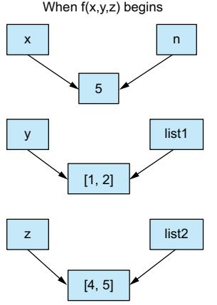
To see what this means, look at the following simple code:
If you’re thinking of variables as containers, this result makes no sense. How could changing the contents of one container simultaneously change the other two? However, if variables are just labels referring to objects, it makes sense that changing the object that all three labels refer to would be reflected everywhere.
If the variables are referring to constants or immutable values, this distinction isn’t quite as clear:
a =1b = ac = bb =5print(a, b, c)#> 1 5 1
Because the objects they refer to can’t change, the behavior of the variables in this case is consistent with either explanation. In fact, in this case, after the third line, a, b, and c all refer to the same unchangeable integer object with the value 1. The next line, b = 5, makes b refer to the integer object 5 but doesn’t change the references of a or c.
Python variables can be set to any object, whereas in C and many other languages, variables can store only the type of value they’re declared as. The following is perfectly legal Python code:
x ="Hello"print(x)#> Hello
x =5print(x)#> 5
x starts out referring to the string object “Hello” and then refers to the integer object 5. Of course, this feature can be abused, because arbitrarily assigning the same variable name to refer successively to different data types can make code confusing.
A new assignment overrides any previous assignments. The del statement deletes the variable (but not necessarily the object it was attached to). Trying to print the variable’s object after deleting it results in an error, as though the variable had never been created in the first place:
x =5print(x)#> 5
del xprint(x)
---------------------------------------------------------------------------
NameError Traceback                                 (most recent call last)
<ipython-input-2-260d38800877> in <cell line: 5>()
 3
 4 del x
----> 5 print(x)   # <-- Line where error occurs
NameError: name 'x' is not defined   # <-- Name of exception that occurred
Here, you have your first look at a traceback, which is printed when an error, called an exception, has been detected. Notice that when we try to access a variable after we’ve deleted it, there is a line of dashes followed by the name of the exception, a NameError. The traceback has a little arrow —-> pointing to the line with the error. The last line explains the exception that was detected, which in this case is a NameError exception because x is no longer defined or valid after its deletion.
In general, the full dynamic call structure of the existing function at the time of the error’s occurrence is returned. If you’re using another Python environment, you might obtain the same information with some small differences. The traceback could look something like the following:
Traceback (most recent call last):
 File "/home/naomi/Dropbox/QPB4/code/vscode/ch04.py", line 5, in <module>
 print(x)
 ^   # <-- Error location indicated with a ^ under the problem
NameError: name 'x' is not defined
This format is a bit simpler, with just a ^ under the error on the next line, but the same information is there.
Chapter 14 describes this mechanism in more detail. A full list of the possible exceptions and what causes them is in the Python standard library documentation. Use the index to find any specific exception (such as NameError) you receive.
4.4 Optional type hints in Python
While Python does not require that you specify types for variables (and function parameters and return values, etc.), current versions of Python do allow you to do so. As mentioned in the previous chapter, in Python many times the type of an object referred to by a variable, or needed as a parameter, or returned by a function or method is not always immediately obvious.
Mixing incompatible types of objects will cause a runtime exception in Python, but it will not raise an error at compile time. Particularly for large projects, there are many times when having the types of objects more explicitly available would be useful. For this, Python has added type hints.
The type hinting notation can be read by type-checking tools like mypy, pyright, pyre, or pytype, as well as several common IDEs, to flag the use of an incompatible or unexpected type. While these tools can report the error, Python itself will not raise a runtime error if the type hints are not followed.
For example, we can create a simple function to add two numbers and use type hinting to indicate that it should only receive and return objects of type int:
def add_ints(x: int, y: int) ->int: # <-- Parameters and return value noted as intsreturn x + yp: int=2.3# <-- Variable p marked as int but set to floatz = add_ints(1, 2)w = add_ints(1.5, 2.5) # <-- Function called with floats
The function definition specifies that both of the parameters and the return value will be of type int. In the first line of code after the function, we specify that the variable p should be of type int but then try to set it to a float. Then the function add_ints is called first with two integers and then with two floats.
If we run this code, Python will execute it without any warning or complaint. However, if we save this code in a file test_types.py and run the mypy checker on that file, three errors will be flagged:
naomi@naomi-NUC:~\$ mypy test_types.py
test\_types.py:4: error: Incompatible types in assignment (expression has
➥type "float", variable has type "int") [assignment]   # <-- Flags setting int variable p to a float
test_types.py:8: error: Argument 1 to "add_ints" has incompatible type
➥"float"; expected "int" [arg-type]   # <-- Flags calling function with two floats instead of ints
test_types.py:8: error: Argument 2 to "add_ints" has incompatible type
➥"float"; expected "int" [arg-type]   # <-- Flags calling function with two floats instead of ints
Found 3 errors in 1 file (checked 1 source file)
When you run the mypy type checker on this code, it reports an error with setting the variable p to 2.3, not because 2.3 is a bad value for p but because the annotation indicated that it should be an int. It also flags two errors in the second call to add_ints, since both of the parameters are floats, but the function is marked as taking two ints. In both cases, Python will run the code without complaint, but the things marked by mypy indicate some confusion between intention and actual use, and that confusion is likely to lead to bugs later on.
4.4.1 Why use type hints?
One reason that type hints are increasingly used is that they help reduce confusion as to what type is expected, in many situations. In a large codebase, it can be particularly frustrating to hunt a bug where an unexpected type of object is returned. Type hints allow many such situations to be caught and fixed before runtime. Type information also allows many editors and IDEs to warn about such errors and suggest appropriate alternatives during the coding process.
4.4.2 Why not use type hints?
While type hints can be useful in many situations, there are situations where they may not be worth the trouble:
In smaller, more informal scripts, it may not be worth the extra time and effort to add type hints.
Trying to fully and explicitly type hint everything in a program may make function or method definitions harder to read. In that case, a decision needs to be made on the tradeoff between human readability and completeness of typing.
Beware of going too far down the type-hinting rabbit hole. Spending too much time obsessed with detailed type hints may not be productive.
Going back and changing working code solely to add type hints also may not be the best use of your time. It’s usually wiser to leave working code alone unless you have a good reason to change it. Adding type hints can be done in the course of other maintenance or refactoring.
4.4.3 Progressive typing
Fortunately, since type hints are optional, you don’t have to add type hints for everything all at once. If you have decided it’s a good idea to use type hints, you can add them progressively, starting with the places where having the type information handy will do the most good.
In this text, we will not routinely use type hints in the short code examples, but we will use them in some of the longer examples and answers to the lab exercises.
4.5 Expressions
Python supports arithmetic and similar expressions; these expressions will be familiar to most readers. The following code calculates the average of 3 and 5, leaving the result in the variable z:
x =3y =5z = (x + y) /2
Note that arithmetic operators involving only integers do not always return an integer. Even though all the values are integers, division (starting with Python 3) returns a floating-point number, so the fractional part isn’t truncated. If you want traditional integer division returning an integer, you can use // instead.
Standard rules of arithmetic precedence apply. If you’d left out the parentheses in the last line, the code would’ve been calculated as x + (y / 2).
Expressions don’t have to involve just numerical values; strings, Boolean values, and many other types of objects can be used in expressions in various ways. I discuss these objects in more detail as they’re used.
Try this: Variables and expressions
In a Jupyter notebook, create some variables. What happens when you try to put spaces, dashes, or other nonalphanumeric characters in the variable name? Play around with a few complex expressions, such as x = 2 + 4 * 5 – 6 / 3. Use parentheses to group the numbers in different ways and see how the result changes compared with the original ungrouped expression.
4.6 Strings
You’ve already seen that Python, like most other programming languages, indicates strings through the use of double quotes. This line leaves the string “Hello, World” in the variable x:
x ="Hello, World"
Backslashes can be used to escape characters—to give them special meanings. \n means the newline character, \t means the tab character, \\ means a single normal backslash character, and \" is a plain double-quote character. It doesn’t end the string:
x ="\tThis string starts with a \"tab\"."x ="This string contains a single backslash(\\)."
You can use single quotes instead of double quotes. The following two lines do the same thing:
x ="Hello, World"x ='Hello, World'
The only difference is that you don’t need to backslash ” characters in single-quoted strings or ’ characters in double-quoted strings:
x ="Don't need a backslash"x ='Can\'t get by without a backslash'x ="Backslash your \" character!"x ='You can leave the " alone'
You can’t split a normal string across lines. This code won’t work:
# This Python code will cause an ERROR -- you can't # split the string across two lines.x ="This is a misguided attempt toput a newline into a string without using backslash-n"
File "<ipython-input-3-dc07520d5086>", line 2
 x = "This is a misguided attempt to
 ^
SyntaxError: unterminated string literal (detected at line 2)
But Python offers triple-quoted strings, which let you have multiline strings and include single and double quotes without backslashes:
x ="""Starting and ending a string with triple " or ' characterspermits embedded newlines, and the use of " and ' withoutbackslashes"""
Now x is the entire sentence between the """ delimiters. [You can use triple single quotes (''') instead of triple double quotes to do the same thing.]
Python offers enough string-related functionality that chapter 6 is devoted to the topic.
4.7 Numbers
Because you’re probably familiar with standard numeric operations from other languages, this book doesn’t contain a separate chapter describing Python’s numeric abilities. This section describes the unique features of Python numbers, and the Python documentation lists the available functions.
Python offers four kinds of numbers: integers, floats, complex numbers, and Booleans. An integer constant is written as an integer—0, –11, +33, 123456—and has unlimited range, restricted only by the resources of your machine. A float can be written with a decimal point or in scientific notation: 3.14, –2E-8, 2.718281828. The precision of these values is governed by the underlying machine but is typically equal to double (64-bit) types in C. Complex numbers are probably of limited interest and are discussed separately later in the section. Booleans are either True or False and behave identically to 1 and 0 except for their string representations.
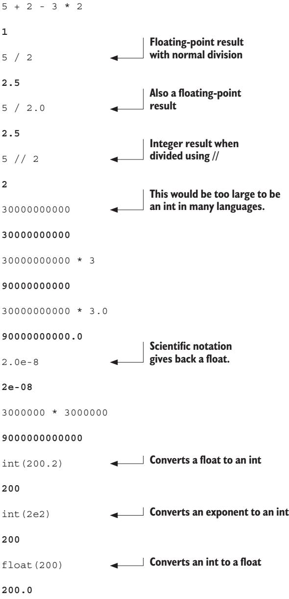
Arithmetic is much like it is in C. Operations involving two integers produce an integer, except for division (/), which results in a float. If the // division symbol is used, the result is an integer, rounding down. Operations involving a float always produce a float. Here are a few examples:
The last three commands are explicit conversions between types. Note that converting from a float to an int will truncate the value and discard the decimal portion. On the other hand, converting an int to a float will always add a .0.
Numbers in Python have two advantages over C or Java: integers can be arbitrarily large, and the division of two integers results in a float.
4.7.1 Built-in numeric functions
Python provides the following number-related functions as part of its core:
See the documentation for the details of how each works.
4.7.2 Advanced numeric functions
More advanced numeric functions, such as the trig and hyperbolic trig functions, as well as a few useful constants, aren’t built into Python but are provided in a standard module called math. I explain modules in detail later. For now, it’s sufficient to know that you must make the math functions in this section available by starting your Python program or interactive session with the statement
from math import*
The math module provides the following functions and constants:
The core Python installation isn’t well suited to intensive numeric computation because of speed constraints. But the powerful Python extension NumPy provides highly efficient implementations of many advanced numeric operations. The emphasis is on array operations, including multidimensional matrices and more advanced functions such as the fast Fourier transform. You should be able to find NumPy (or links to it) at www.scipy.org.
4.7.4 Complex numbers
Complex numbers are created automatically whenever an expression of the form nj is encountered, with n having the same form as a Python integer or float. j is, of course, standard notation for the imaginary number equal to the square root of –1, for example:
(3+2j)#> (3+2j)
Note that Python expresses the resulting complex number in parentheses as a way of indicating that what’s printed to the screen represents the value of a single object:
Calculating j * j gives the expected answer of –1, but the result remains a Python complex-number object. Complex numbers are never converted automatically to equivalent real or integer objects. But you can easily access their real and imaginary parts with real and imag:
z = (3+5j)z.real#> 3.0z.imag#> 5.0
Note that real and imaginary parts of a complex number are always returned as floating-point numbers.
4.7.5 Advanced complex-number functions
The functions in the math module don’t apply to complex numbers; the rationale is that most users want the square root of –1 to generate an error, not an answer! Instead, similar functions, which can operate on complex numbers, are provided in the cmath module:
acos, acosh, asin, asinh, atan, atanh, cos, cosh, e, exp, log, log10,
pi, sin, sinh, sqrt, tan, tanh.
To make clear in the code that these functions are special-purpose complex-number functions and to avoid name conflicts with the more normal equivalents, it’s best to import the cmath module with
import cmath
and then to explicitly refer to the cmath package when using the function:
import cmathcmath.sqrt(-1)#> 1j
Minimizing from import *
This is a good example of why it’s best to minimize the use of the from import * form of the import statement. If you used it to import first the math module and then the cmath module, the commonly named functions in cmath would override those of math. It’s also more work for someone reading your code to figure out the source of the specific functions you use. Some modules are explicitly designed to use this form of import.
See chapter 10 for more details on how to use modules and module names.
The important thing to keep in mind is that by importing the cmath module, you can do almost anything with complex numbers that you can do with other numbers.
Try this: Manipulating strings and numbers
In a Jupyter notebook, create some string and number variables (integers, floats, and complex numbers). Experiment a bit with what happens when you do operations with them, including across types. Can you multiply a string by an integer, for example, or can you multiply it by a float or complex number? Also load the math module and try a few of the functions; then load the cmath module and do the same. What happens if you try to use one of those functions on an integer or float after loading the cmath module? How might you get the math module functions back?
4.8 The None value
In addition to standard types such as strings and numbers, Python has a special basic data type that defines a single special data object called None. As the name suggests, None is used to represent an empty value. It appears in various guises throughout Python. For example, a procedure in Python is just a function that doesn’t explicitly return a value, which means that, by default, it returns None.
None is often useful in day-to-day Python programming as a placeholder to indicate a point in a data structure where meaningful data will eventually be found, even though that data hasn’t yet been calculated. You can easily test for the presence of None because there’s only one instance of None in the entire Python system (all references to None point to the same object), and None is equivalent only to itself.
4.9 Getting input from the user
You can use the input() function to get input from the user. Use the prompt string you want to display to the user as input’s parameter:
name =input("Name? ")
Name? Jane
print(name)#> Jane
age =int(input("Age? ")) # <-- Converts input from a string to an int
Age? 28
print(age)#> 28
This is a fairly simple way to get user input. The one catch is that the input comes in as a string, so if you want to use it as a number, you have to use the int() or float() function to convert it to an int or float.
Try this: Getting input
Experiment with the input() function to get string and integer input. Using code similar to the previous code, what is the effect of not using int() around the call to input()for integer input? Can you modify that code to accept a float—say, 28.5? What happens if you deliberately enter the wrong type of value? Examples include a float in which an integer is expected and a string in which a number is expected—and vice versa.
4.10 Built-in operators
Python provides various built-in operators, from the standard (+, *, and so on) to the more esoteric, such as operators for performing bit shifting, bitwise logical functions, and so forth. Most of these operators are no more unique to Python than to any other language; hence, I won’t explain them in the main text. You can find a complete list of the Python built-in operators in the documentation.
4.11 Basic Python style
Python has relatively few limitations on coding style with the obvious exception of the requirement to use indentation to organize code into blocks. Even in that case, the amount of indentation and type of indentation (tabs versus spaces) isn’t mandated. However, there are preferred stylistic conventions for Python, contained in Python Enhancement Proposal (PEP) 8, which is summarized in appendix A and available online at www.python.org/dev/peps/pep-0008/. A selection of Pythonic conventions is provided in table 4.1, but to fully absorb Pythonic style, periodically reread PEP 8.
Table 4.1 Pythonic coding conventions
Situation
Suggestion
Example
Module/package names
Short, all lowercase, underscores only if needed
imp, sys
Function names
All lowercase, underscores_for_readablitiy
foo(), my_func()
Variable names
All lowercase, underscores_for_readablitiy
my_var
Class names
CapitalizeEachWord
MyClass
Constant names
ALL_CAPS_WITH_UNDERSCORES
PI, TAX_RATE
Indentation
Four spaces per level, no tabs
Comparisons
Don’t compare explicitly to True or False.
if my_var: if not my_var:
I strongly urge you to follow the conventions of PEP 8. They’re wisely chosen and time tested, and they’ll make your code easier for you and other Python programmers to understand.
Quick check: Pythonic style
Which of the following variable and function names do you think are not good Pythonic style? Why?
Python code is organized by using levels of indentation.
Python comments can be marked with an initial # character.
Strings in triple quotes at the beginning of a module, function, or method are “docstrings,” which explain what the object does and/or how it behaves.
The intended types of variables, parameters, and function return values can optionally be marked using Python’s type hints.
Python has the usual data types for strings and numbers, as well as data structures like lists, tuples, sets, and dictionaries.
The input() function can be used to get input from the user as a string.
Python has several built-in operators, including +, -, /, //, %, *, etc.
The preferred Python style can be found in PEP 8 in the online Python documentation.
5. Lists, tuples, and sets
This chapter covers
Manipulating lists and list indices
Modifying lists
Sorting
Using common list operations
Handling nested lists and deep copies
Using tuples
Creating and using sets
In this chapter, I discuss the two major Python sequence types: lists and tuples. At first, lists may remind you of arrays in many other languages, but don’t be fooled: lists are a good deal more flexible and powerful than plain arrays.
Tuples are like lists that can’t be modified; you can think of them as a restricted type of list or as a basic record type. I discuss the need for such a restricted data type later in the chapter. This chapter also discusses another Python collection type: sets. Sets are useful when an object’s membership in the collection, as opposed to its position, is important.
Most of the chapter is devoted to lists, because if you understand lists, you pretty much understand tuples. The last part of the chapter discusses the differences between lists and tuples in both functional and design terms.
5.1 Lists are like arrays
A list in Python is similar to an array in Java or C or any other language; it’s an ordered collection of objects. You create a list by enclosing a comma-separated list of elements in square brackets, as follows:
# This assigns a three-element list to xx = [1, 2, 3]
Note that you don’t have to worry about declaring the list or fixing its size ahead of time. This line creates the list as well as assigns it, and a list automatically grows or shrinks as needed.
Arrays in Python
A typed array module available in Python provides arrays based on C data types. Information on its use can be found in the documentation for the Python standard library. I suggest that you look into it only if you really need performance improvement. If a situation calls for numerical computations, you should consider using NumPy, mentioned in chapter 4 and available at www.scipy.org/.
Unlike lists in many other languages, Python lists can contain different types of elements; a list element can be any Python object. The following is a list that contains a variety of elements:
# First element is a number, second is a string, third is another list.x = [2, "two", [1, 2, 3]]
Probably the most basic built-in list function is the len function, which returns the number of elements in a list:
x = [2, "two", [1, 2, 3]]len(x)#> 3
Note that the len function doesn’t count the items in the inner, nested list.
Quick check: len()
What would len() return for each of the following? [0]; []; [[1, 3, [4, 5], 6], 7]
5.2 List indices
Understanding how list indices work will make Python much more useful to you. Please read the whole section!
Elements can be extracted from a Python list by using a notation like C’s array indexing. Like C and many other languages, Python starts counting from 0; asking for element 0 returns the first element of the list, asking for element 1 returns the second element, and so forth. The following are a few examples:
x = ["first", "second", "third", "fourth"]x[0]#> 'first'x[2]#> 'third'
But Python indexing is more flexible than C indexing. If indices are negative numbers, they indicate positions counting from the end of the list, with –1 being the last position in the list, –2 being the second-to-last position, and so forth. Continuing with the same list x, you can do the following:
a = x[-1]a#> 'fourth'x[-2]#> 'third'
For operations involving a single list index, it’s generally satisfactory to think of the index as pointing at a particular element in the list. For more advanced operations, it’s more correct to think of list indices as indicating positions between elements. In the list [“first”, “second”, “third”, “fourth”], you can think of the indices as pointing as follows.
x =[
“first”,
“second”,
“third”,
“fourth”
]
Positive indices
0
1
2
3
Negative indices
–4
–3
–2
–1
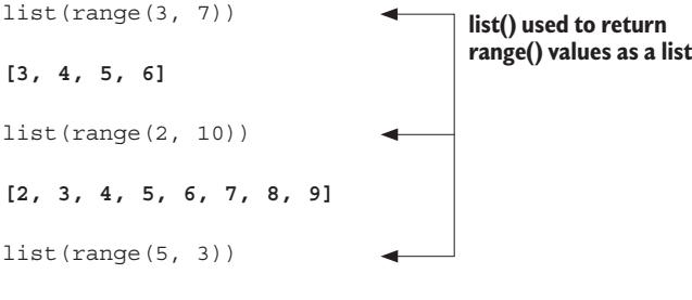
This is irrelevant when you’re extracting a single element, but Python can extract or assign to an entire sublist at once—an operation known as slicing. Instead of entering list[index] to extract the item just after index, enter list[index1:index2] to extract all items, including index1 and up to (but not including) index2, into a new list. The following are some examples:
It may seem reasonable that if the second index indicates a position in the list before the first index, this code would return the elements between those indices in reverse order, but this isn’t what happens. Instead, this code returns an empty list:
x[-1:2]
#> []
When slicing a list, it’s also possible to leave out index1 or index2. Leaving out index1 means “Go from the beginning of the list,” and leaving out index2 means “Go to the end of the list”:
Omitting both indices makes a new list that goes from the beginning to the end of the original list—that is, copies the list. This technique is useful when you want to make a copy that you can modify without affecting the original list:
Using what you know about the len() function and list slices, how would you combine the two to get the second half of a list when you don’t know what size it is? Experiment in the Python shell to confirm that your solution works.
5.3 Modifying lists
You can use list index notation to modify a list as well as to extract an element from it. Put the index on the left side of the assignment operator:
x = [1, 2, 3, 4]x[1] ="two"x#> [1, 'two', 3, 4]
Slice notation can be used here too. Saying something like lista[index1:index2] = listb causes all elements of lista between index1 and index2 to be replaced by the elements in listb. listb can have more or fewer elements than are removed from lista, in which case the length of lista is altered. You can use slice assignment to do several things, as shown in the following:
x = [1, 2, 3, 4]x[len(x):] = [5, 6, 7] # <-- Appends a list to end of a listx#> [1, 2, 3, 4, 5, 6, 7]x[:0] = [-1, 0] # <-- Appends a list to front of a listx#> [-1, 0, 1, 2, 3, 4, 5, 6, 7]x[1:-1] = [] # <-- Removes elements from a listx#> [-1, 7]
Appending a single element to a list is such a common operation that there’s a special append method for it:
x = [1, 2, 3]x.append("four")x#> [1, 2, 3, 'four']
One problem can occur if you try to append one list to another. The list gets appended as a single element of the main list:
There’s also a special insert method to insert new list elements between two existing elements or at the front of the list. insert is used as a method of a list object and takes two additional arguments. The first additional argument is the index position in the list where the new element should be inserted, and the second is the new element itself:
insert understands list indices as discussed in section 5.2, but for most uses, it’s easiest to think of list.insert(n, elem) as meaning insert elem just before the nth element of the list. insert is just a convenience method. Anything that can be done with insert can also be done with slice assignment. That is, list.insert(n, elem) is the same thing as list[n:n] = [elem] when n is nonnegative. Using insert makes for somewhat more readable code, and insert even handles negative indices:
x = [1, 2, 3]x.insert(-1, "hello")print(x)#> [1, 2, 'hello', 3]
The del statement is the preferred method of deleting list items or slices. It doesn’t do anything that can’t be done with slice assignment, but it’s usually easier to remember and easier to read:
In general, del list[n] does the same thing as list[n:n+1] = [], whereas del list[m:n] does the same thing as list[m:n] = [].
The remove method isn’t the inverse of insert. Whereas insert inserts an element at a specified location, remove looks for the first instance of a given value in a list and removes that value from the list:
x = [1, 2, 3, 4, 3, 5]x.remove(3)x#> [1, 2, 4, 3, 5]x.remove(3)x#> [1, 2, 4, 5]x.remove(3)#> ---------------------------------------------------------------------------#> ValueError Traceback (most recent call last)#> <ipython-input-9-be7b9eddb459> in <cell line: 1>()#> ----> 1 x.remove(3) #> ValueError: list.remove(x): x not in list
If remove can’t find anything to remove, it raises an error. You can catch this error by using the exception-handling abilities of Python, or you can avoid the problem by using in to check for the presence of something in a list before attempting to remove it (see section 5.5.1 for examples of in).
The reverse method is a more specialized list modification method. It efficiently reverses a list in place:
x = [1, 3, 5, 6, 7]x.reverse()x#> [7, 6, 5, 3, 1]
Try this: Modifying lists
Suppose that you have a list of 10 items. How might you move the last three items from the end of the list to the beginning, keeping them in the same order?
5.4 Sorting lists
Lists can be sorted by using the built-in Python sort method:
This method does an in-place sort—that is, changes the list being sorted. To sort a list without changing the original list, you have two options. You can use the sorted() built-in function, discussed in section 5.4.2, or you can make a copy of the list and sort the copy:
x = [2, 4, 1, 3]y = x[:] # <-- A full list slice makes a copy of the list.y.sort() # <-- Sorts method on copy, not originaly#> [1, 2, 3, 4]x#> [2, 4, 1, 3]
Note that here we used the [:] notation to make a slice of the entire list. Since slicing creates a new list, this in effect creates a copy of the entire list, which we can then sort using the sort() method.
Sorting works with strings too:
x = ["Life", "Is", "Enchanting"]x.sort()x#> ['Enchanting', 'Is', 'Life']
The sort method can sort just about anything because Python can compare just about anything. But there’s one caveat in sorting: the default key method used by sort requires all items in the list to be of comparable types. That means that using the sort method on a list containing both numbers and strings raises an exception:
x = [1, 2, 'hello', 3]x.sort()#> ---------------------------------------------------------------------------#> TypeError Traceback (most recent call last)#> <ipython-input-8-9c6228d80c69> in <cell line: 2>()#> 1 x = [1, 2, 'hello', 3]#> ----> 2 x.sort()#> 3 #> TypeError: '<' not supported between instances of 'str' and 'int'
According to the built-in Python rules for comparing complex objects, the sublists are sorted first by the ascending first element and then by the ascending second element.
sort is even more flexible; it has an optional reverse parameter that causes the sort to be in reverse order when reverse=True, and it’s possible to use your own key function to determine how elements of a list are sorted.
5.4.1 Custom sorting
To use custom sorting, you need to be able to define functions—something I haven’t talked about yet. In this section, I also discuss the fact that len(string) returns the number of characters in a string. String operations are discussed more fully in chapter 6.
By default, sort uses built-in Python comparison functions to determine ordering, which is satisfactory for most purposes. At times, though, you want to sort a list in a way that doesn’t correspond to this default ordering. Suppose you want to sort a list of words by the number of characters in each word, as opposed to the lexicographic sort that Python normally carries out.
To do this, write a function that returns the value, or key, that you want to sort on and use it with the sort method. That function in the context of sort is a function that takes one argument and returns the key or value that the sort function is to use.
For number-of-characters ordering, a suitable key function could be
def num_of_chars(string1):returnlen(string1)
This key function is trivial. It passes the length of each string back to the sort method, rather than the strings themselves.
After you define the key function, using it is a matter of passing it to the sort method by using the key keyword. Because functions are Python objects, they can be passed around like any other Python objects. Here’s a small program that illustrates the difference between a default sort and your custom sort:
The first list is in lexicographical order (with uppercase coming before lowercase), and the second list is ordered by ascending number of characters.
It’s also possible to use an anonymous lambda function in the sort() call itself. This can be handy if the sort function is very short (which it usually is) and only used for sorting (again, as it should be). The code using the function comp_num_of_chars could also be written with a lambda function as
word_list.sort(key=lambda x: len(x))
The lambda is defined with three elements: a variable for the parameter, in this case x; a colon; and the return value, in this example len(x). For simple functions with only a simple return value, a lambda function saves having to create more function names, and you can see how the sort key works without having to look at the function elsewhere.
Custom sorting is very useful, but if performance is critical, it may be slower than the default. Usually, this effect is minimal, but if the key function is particularly complex, the effect may be more than desired, especially for sorts involving hundreds of thousands or millions of elements.
One particular place to avoid custom sorts is where you want to sort a list in descending, rather than ascending, order. In this case, use the sort method’s reverse parameter set to True. If for some reason you don’t want to do that, it’s still better to sort the list normally and then use the reverse method to invert the order of the resulting list. These two operations together—the standard sort and the reverse—will still be much faster than a custom sort.
5.4.2 The sorted () function
Lists have a built-in method to sort themselves, but other iterables in Python, such as the keys of a dictionary, don’t have a sort method. Python also has the built-in function sorted(), which returns a sorted list from any iterable. sorted() uses the same key and reverse parameters as the sort method:
x = (4, 3, 1, 2)y =sorted(x)y#> [1, 2, 3, 4] z =sorted(x, reverse=True)z#> [4, 3, 2, 1]
Try this: Sorting lists
Suppose that you have a list in which each element is in turn a list: [[1, 2, 3], [2, 1, 3], [4, 0, 1]]. If you wanted to sort this list by the second element in each list so that the result would be [[4, 0, 1], [2, 1, 3], [1, 2, 3]], what function would you write to pass as the key value to the sort() method?
5.5 Other common list operations
Several other list methods are frequently useful, but they don’t fall into any specific category.
5.5.1 List membership with the in operator
It’s easy to test whether a value is in a list by using the in operator, which returns a Boolean value. You can also use the inverse: the not in operator:
3in [1, 3, 4, 5]#> True
3notin [1, 3, 4, 5]#> False
3in ["one", "two", "three"]#> False
3notin ["one", "two", "three"]#> True
5.5.2 List concatenation with the + operator
To create a list by concatenating two existing lists, use the + (list concatenation) operator, which leaves the argument lists unchanged:
z = [1, 2, 3] + [4, 5]z#> [1, 2, 3, 4, 5]
5.5.3 List initialization with the * operator
Use the * operator to produce a list of a given size, which is initialized to a given value. This operation is a common one for working with large lists whose size is known ahead of time. Although you can use append to add elements and automatically expand the list as needed, you obtain greater efficiency by using * to correctly size the list at the start of the program. A list that doesn’t change in size doesn’t incur any memory reallocation overhead:
z = [None] *4z#> [None, None, None, None]
When used with lists in this manner, * (which in this context is called the list multiplication operator) replicates the given list the indicated number of times and joins all the copies to form a new list. This is the standard Python method for defining a list of a given size ahead of time. A list containing a single instance of None is commonly used in list multiplication, but the list can be anything:
z = [3, 1] *2z#> [3, 1, 3, 1]
5.5.4 List minimum or maximum with min and max
You can use min and max to find the smallest and largest elements in a list. You’ll probably use min and max mostly with numerical lists, but you can use them with lists containing any type of element. Trying to find the maximum or minimum object in a set of objects of different types causes an error if comparing those types doesn’t make sense:
min([3, 7, 0, -2, 11])#> -2
max([4, "Hello", [1, 2]])#> ---------------------------------------------------------------------------#> TypeError Traceback (most recent call last)#> <ipython-input-7-15ab1869d5d5> in <cell line: 1>()#> ----> 1 max([4, "Hello", [1, 2]])#> TypeError: '>' not supported between instances of 'str' and 'int'
5.5.5 List search with index
If you want to find where in a list a value can be found (rather than wanting to know only whether the value is in the list), use the index method. This method searches through a list looking for a list element equivalent to a given value and returns the position of that list element:
x = [1, 3, "five", 7, -2]x.index(7)#> 3x.index(5)#> ---------------------------------------------------------------------------#> ValueError Traceback (most recent call last)#> <ipython-input-6-96ad5df81983> in <cell line: 1>()#> ----> 1 x.index(5)#> ValueError: 5 is not in list
Attempting to find the position of an element that doesn’t exist in the list raises an error, as shown here. This error can be handled in the same manner as the analogous error that can occur with the remove method (that is, by testing the list with in before using index).
5.5.6 List matches with count
count also searches through a list, looking for a given value, but it returns the number of times that the value is found in the list rather than positional information:
You can see that lists are very powerful data structures, with possibilities that go far beyond those of plain old arrays. List operations are so important in Python programming that it’s worth laying them out for easy reference, as shown in table 5.1.
Table 5.1 List operations
List operation
Explanation
Example
[]
Creates an empty list
x = []
len
Returns the length of a list
len(x)
append
Adds a single element to the end of a list
x.append('y')
extend
Adds another list to the end of the list
x.extend(['a', 'b'])
insert
Inserts a new element at a given position in the list
x.insert(0, 'y')
del
Removes a list element or slice
del(x[0])
remove
Searches for and removes a given value from a list
x.remove('y')
reverse
Reverses a list in place
x.reverse()
sort
Sorts a list in place
x.sort()
+
Adds two lists together
x1 + x2
*
Replicates a list
x = ['y'] * 3
min
Returns the smallest element in a list
min(x)
max
Returns the largest element in a list
max(x)
index
Returns the position of a value in a list
x.index['y']
count
Counts the number of times a value occurs in a list
x.count('y')
sum
Sums the items (if they can be summed)
sum(x)
in
Returns whether an item is in a list
'y' in x
Being familiar with these list operations will make your life as a Python coder much easier.
Quick check: List operations
What would be the result of len([[1,2]] * 3)? What are two differences between using the in operator and a list’s index() method? Which of the following will raise an exception? min(["a", "b", "c"]); max([1, 2, "three"]); [1, 2, 3].count("one")
Try this: List operations
If you have a list x, write the code to safely remove an item if—and only if—that value is in the list. Modify that code to remove the element only if the item occurs in the list more than once.
5.6 Nested lists and deep copies
This section covers another advanced topic that you may want to skip if you’re just learning the language.
Lists can be nested. One application of nesting is to represent two-dimensional matrices. The members of these matrices can be referred to by using two-dimensional indices. Indices for these matrices work as follows:
This mechanism scales to higher dimensions in the manner you’d expect.
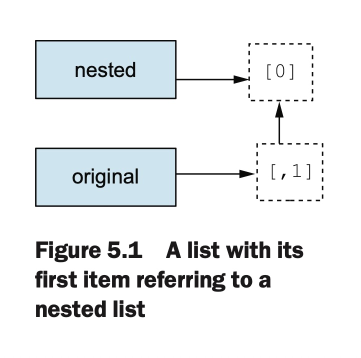
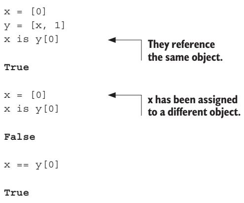
Most of the time, this is all you need to concern yourself with. But you may run into a problem with nested lists—specifically, the way that variables refer to objects and how some objects (such as lists) can be modified (are mutable). An example is the best way to illustrate:
But if nested is set to another list, the connection between them is broken:
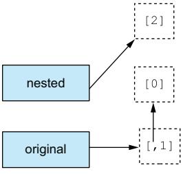
nested = [2]original#> [[0], 1]
Figure 5.2 illustrates this condition.
Figure 5.2 The first item of the original list is still a nested list, but the nested variable refers to a different list.
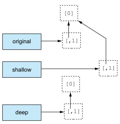
You’ve seen that you can obtain a copy of a list by taking a full slice (that is, x[:]). You can also obtain a copy of a list by using the + or * operators (for example, x + [] or x * 1). These techniques are slightly less efficient than the slice method. All three create what is called a shallow copy of the list, which is probably what you want most of the time. But if your list has other lists nested in it, you may want to make a deep copy. You can do this with the deepcopy function of the copy module:
original = [[0], 1]shallow = original[:]import copydeep = copy.deepcopy(original)
See figure 5.3 for an illustration.
Figure 5.3 A deep copy copies nested lists.
The lists pointed at by the original or shallow variables are connected. Changing the value in the nested list through either one of them affects the other:
This behavior is the same for any other nested objects in a list that are modifiable (such as dictionaries).
Now that you’ve seen what lists can do, it’s time to look at tuples.
Try this: List copies
Suppose that you have the following list: x = [[1, 2, 3], [4, 5, 6], [7, 8, 9]] What code could you use to get a copy y of that list in which you could change the elements without the side effect of changing the contents of x?
5.7 Tuples
Tuples are data structures that are very similar to lists, but they can’t be modified; they can only be created. Tuples are so much like lists that you may wonder why Python bothers to include them. The reason is that tuples have important roles that can’t be efficiently filled by lists, such as keys for dictionaries.
5.7.1 Tuple basics
Creating a tuple is similar to creating a list: assign a sequence of values to a variable. A list is a sequence that’s enclosed by [ and ]; a tuple is a sequence that’s enclosed by ( and ):
x = ('a', 'b', 'c')
This line creates a three-element tuple.
After a tuple is created, using it is so much like using a list that it’s easy to forget that tuples and lists are different data types:
The main difference between tuples and lists is that tuples are immutable. An attempt to modify a tuple results in a confusing error message, which is Python’s way of saying that it doesn’t know how to set an item in a tuple:
x[2] ='d'#> ---------------------------------------------------------------------------#> TypeError Traceback (most recent call last)#> <ipython-input-2-dcc4b983047e> in <cell line: 1>()#> ----> 1 x[2] = 'd'#> TypeError: 'tuple' object does not support item assignment
You can create tuples from existing ones by using the + and * operators:
Tuples themselves can’t be modified. But if a tuple contains any mutable objects (for example, lists or dictionaries), these objects may be changed if they’re still assigned to their own variables. Tuples that contain mutable objects aren’t allowed as keys for dictionaries.
Copying tuples
Because tuples can’t be modified, the shallow copy methods shown here don’t return new objects but aliases pointing to the same object. This is true not only for tuples but also for string and byte objects, which are covered in the next chapter. In practice you can still think of these aliases as “copies” since there is nothing you could do with a true copy that you can’t also do with an alias (and aliases are much faster and more memory efficient).
5.7.2 One-element tuples need a comma
A small syntactical point is associated with using tuples. Because the square brackets used to enclose a list aren’t used elsewhere in Python, it’s clear that [] means an empty list and that [1] means a list with one element. The same thing isn’t true of the parentheses used to enclose tuples. Parentheses can also be used to group items in expressions to force a certain evaluation order. If you say (x + y) in a Python program, do you mean that x and y should be added and then put into a one-element tuple, or do you mean that the parentheses should be used to force x and y to be added before any expressions to either side come into play?
This situation is a problem only for tuples with one element because tuples with more than one element always include commas to separate the elements, and the commas tell Python that the parentheses indicate a tuple, not a grouping. In the case of oneelement tuples, Python requires that the element in the tuple be followed by a comma to disambiguate the situation. In the case of zero-element (empty) tuples, there’s no problem. An empty set of parentheses must be a tuple because it’s meaningless otherwise:
x =3y =4(x + y) # This line adds x and y.#> 7(x + y,) # Including a comma indicates that the parentheses denote a tuple.#> (7,)() # To create an empty tuple, use an empty pair of parentheses.#> ()
5.7.3 Packing and unpacking tuples
As a convenience, Python permits tuples of variables to appear on the left side of an assignment operator, in which case variables in the tuple receive the corresponding values from the tuple on the right side of the assignment operator. The following is a simple example:
This example can be written even more simply because Python recognizes tuples in an assignment context even without the enclosing parentheses. The values on the right side are packed into a tuple and then unpacked into the variables on the left side:
one, two, three, four =1, 2, 3, 4
One line of code has replaced the following four lines of code:
one =1two =2three =3four =4
This technique is a convenient way to swap values between variables. Instead of saying
temp = var1var1 = var2var2 = temp
simply say
var1, var2 = var2, var1
To make things even more convenient, Python 3 has an extended unpacking feature, allowing an element marked with * to absorb any number of elements not matching the other elements. Again, some examples make this feature clearer:
Note that the starred element receives all the surplus items as a list and that if there are no surplus elements, the starred element receives an empty list.
Packing and unpacking can also be performed with lists:
def greet(first, last, age):print(f"{first}{last} is {age} years old")# * : 위치 인자로 전달args = ['Alice', 'Smith', 30]greet(*args) # greet('Alice', 'Smith', 30)과 동일# 출력: Alice Smith is 30 years old# ** : 키워드 인자로 전달kwargs = {'first': 'Bob', 'last': 'Jones', 'age': 25}greet(**kwargs) # greet(first='Bob', last='Jones', age=25)와 동일# 출력: Bob Jones is 25 years old# 혼합 사용args = ['Charlie', 'Brown']kwargs = {'age': 35}greet(*args, **kwargs) # greet('Charlie', 'Brown', age=35)# 출력: Charlie Brown is 35 years old
4. 함수 정의에서의 사용
# *args : 가변 위치 인자 받기def sum_all(*args):print(f"받은 인자들: {args}") # 튜플로 받음returnsum(args)print(sum_all(1, 2, 3, 4, 5))# 받은 인자들: (1, 2, 3, 4, 5)# 15# **kwargs : 가변 키워드 인자 받기def print_info(**kwargs):print(f"받은 인자들: {kwargs}") # 딕셔너리로 받음for key, value in kwargs.items():print(f"{key}: {value}")print_info(name='Alice', age=30, city='Seoul')# 받은 인자들: {'name': 'Alice', 'age': 30, 'city': 'Seoul'}# name: Alice# age: 30# city: Seoul# 둘 다 사용def flexible_function(required, *args, **kwargs):print(f"필수 인자: {required}")print(f"추가 위치 인자: {args}")print(f"추가 키워드 인자: {kwargs}")flexible_function(1, 2, 3, 4, x=10, y=20)# 필수 인자: 1# 추가 위치 인자: (2, 3, 4)# 추가 키워드 인자: {'x': 10, 'y': 20}
5. 언패킹 할당
# * : 나머지 요소들 모으기a, *b, c = [1, 2, 3, 4, 5]print(a) # 1print(b) # [2, 3, 4]print(c) # 5first, *middle, last = ['a', 'b', 'c', 'd', 'e']print(first) # 'a'print(middle) # ['b', 'c', 'd']print(last) # 'e'# ** : 딕셔너리에서는 이런 식으로 사용 불가# 딕셔너리는 다른 방식으로 분해person = {'name': 'Alice', 'age': 30, 'city': 'Seoul'}name = person['name']rest = {k: v for k, v in person.items() if k !='name'}print(name) # 'Alice'print(rest) # {'age': 30, 'city': 'Seoul'}
5.7.4 Converting between lists and tuples
Tuples can be easily converted to lists with the list function, which takes any sequence as an argument and produces a new list with the same elements as the original sequence. Similarly, lists can be converted to tuples with the tuple function, which does the same thing but produces a new tuple instead of a new list:
As an interesting side note, list is a convenient way to break a string into characters:
list("Hello")#> ['H', 'e', 'l', 'l', 'o']
This technique works because list (and tuple) apply to any Python sequence, and a string is just a sequence of characters. (Strings are discussed fully in chapter 6.)
Quick check: Tuples
Explain why the following operations aren’t legal for the tuple x = (1, 2, 3, 4):
x.append(1)x[1] ="hello"del x[2]
If you had a tuple x = (3, 1, 4, 2), how might you end up with x sorted?
5.8 Sets
A set in Python is an unordered collection of objects used when membership and uniqueness in the set are the main things you need to know about that object. Like dictionary keys (discussed in chapter 7), the items in a set must be immutable and hashable. This means that ints, floats, strings, and tuples can be members of a set, but lists, dictionaries, and sets themselves can’t.
5.8.1 Set operations
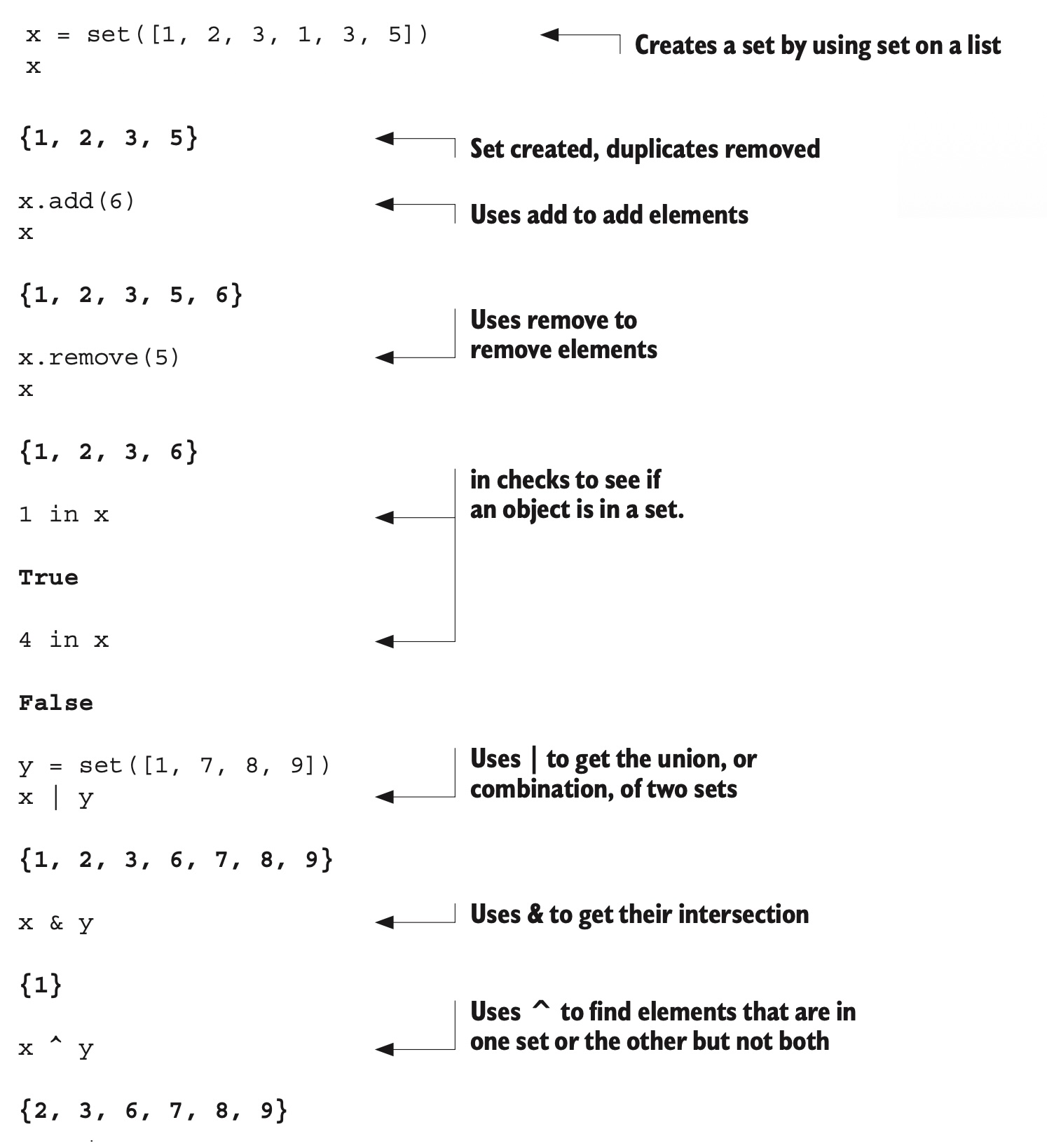
In addition to the operations that apply to collections in general, such as in, len, and iteration in for loops, sets have several set-specific operations:
You can create a set by using set on a sequence, such as a list. When a sequence is made into a set, duplicates are removed. After creating a set by using the set function, you can use add and remove to change the elements in the set. The in keyword is used to check for membership of an object in a set. You can also use | to get the union, or combination, of two sets, & to get their intersection, and ^ to find their symmetric difference—that is, elements that are in one set or the other but not both.
These examples aren’t a complete listing of set operations, but they are enough to give you a good idea of how sets work. For more information, refer to the official Python documentation.
5.8.2 Frozen sets
Because sets aren’t immutable and hashable, they can’t belong to other sets. To remedy that situation, Python has another set type, frozenset, which is just like a set but can’t be changed after creation. Because frozen sets are immutable and hashable, they can be members of other sets:
If you were to construct a set from the following list, how many elements would the set have? [1, 2, 5, 1, 0, 2, 3, 1, 1, (1, 2, 3)]
5.9 Lab: Examining a list
In this lab, the task is to read a set of temperature data (the monthly high temperatures at Heathrow Airport for 1948 through 2016) from a file and then find some basic information: the highest and lowest temperatures, the mean (average) temperature, and the median temperature (the temperature in the middle if all the temperatures are sorted).
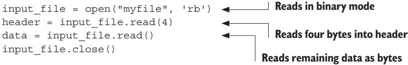
The temperature data is in the file lab_05.txt in the source code directory for this chapter. Because I haven’t yet discussed reading files, here’s the code to read the files into a list:
temperatures = []withopen('lab_05.txt') as infile:for row in infile: temperatures.append(float(row.strip()))
You should find the highest and lowest temperature, the average, and the median. You’ll probably want to use the min(), max(), sum(), len(), and sort() functions/ methods. As a bonus, determine how many unique temperatures are in the list.
5.9.1 Why solve it the old-fashioned way?
You should have a try at creating a solution to this problem using your knowledge and the material presented in this chapter. The preceding code will open a file and read its contents in as a list of floats. You can then use the functions mentioned to get the answers required. And for a bonus, the key is to think of how to convert a list so that only unique values remain.
You may be thinking, “Why should I write this code? Can’t I use AI to generate a solution?” And the answer is yes, you can, but trying to create a solution on your own first helps you both understand the problem better and learn how Python works. Both of those are vital for using an AI code generator—you need a solid understanding of the problem to create an effective prompt for the AI, and a solid understanding of how Python works is essential for evaluating the generated code.
If you are using the Jupyter notebook for this chapter, there is a cell with the code to load the file where you can put in your code to find the mean, median, etc. temperatures. Next, we’ll discuss a sample solution created by a human (me) and compare it to the AI solution.
5.9.2 Solving the problem with AI code generation
As mentioned in chapter 2, there are several AI code generation tools, and the landscape is rapidly evolving, so it’s quite possible you will be using something different from the options available as I write this. For the sake of illustration, I will use the code generator available in Google Colaboratory, which is currently available for free, and GitHub Copilot, which is available by subscription with a free trial and runs in Microsoft’s VS Code IDE. I’ll discuss one of the solutions and note if the other system produces something dramatically different.
Prompt creation
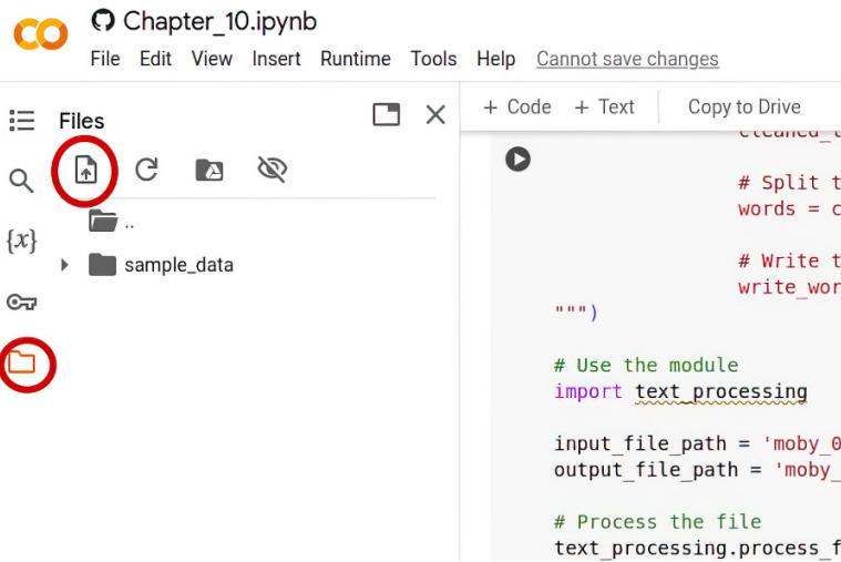
To generate code in Colaboratory, we need to click the generate link shown in an empty cell, “Start coding or generate with AI.” Once we do that, we get a code generation dialog waiting for a prompt telling the code generator what we want to do. Once we enter the prompt in the field after the Using… button (as shown in the following figure), we can click the Generate button to generate our code.
Creating a prompt is an evolving art, but since the prompt field is limited, we can’t simply copy and paste the whole problem statement. Since we already have the code to read the file into a list as a series of floats, our prompt should focus only on what we need the code to do.
With this guidance, you can go ahead and try creating a prompt and generating some code. Try to evaluate the generated code and, if necessary, refine your prompt.
5.9.3 Solutions and discussion
To create our prompt, we focused on what we needed the code to do. The following is the list of things we needed done:
1 Use the list temperatures.
2 Find the high and low temperature.
3 Find the mean and median.
4 State how many unique temperatures there are (yes, let’s do the bonus).
We might combine this into a prompt as
Using the list temperatures, find the high, low, mean, and median temperatures, and show how many unique temperatures are in the list.
This prompt is complete and concise and covers exactly what we need. Remember that we already had the code to load the file, so we don’t need to ask for that, but of course we do need to add that code to the generated code:
temperatures = []withopen('lab_05.txt') as infile:for row in infile: temperatures.append(float(row.strip()))
The human coded solution
The solution I came up with follows.
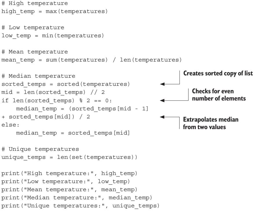
max_temp =max(temperatures)min_temp =min(temperatures)mean_temp =sum(temperatures)/len(temperatures)# we'll need to sort to get the median temptemperatures.sort() # <-- Sorts the temperatures list in placemedian_temp = temperatures[len(temperatures)//2] # <-- Gets value from midpoint of list or one above midpoint if an even number of elementsprint(f"max = {max_temp}")print(f"min = {min_temp}")print(f"mean = {mean_temp}")print(f"median = {median_temp}")# Bonusunique_temps =len(set(temperatures))print(f"number of uniquie temps - {unique_temps}")
This solution does the job and reflects my bias to keep things simple and to keep comments to a minimum.
The AI-generated solution
The code generated by AI is remarkably similar—probably because the problem is not complex. Using Copilot (the Colaboratory code was nearly identical) we get
This code also does the job, with what is arguably nicer formatting and more comments.
The AI version uses more whitespace, which makes the code easier to read. It also uses more comments—to my mind maybe more than needed. It’s good style in Python to use comments only where needed to explain why something is as it is, and in my opinion a comment # High temperature right before the high_temp is not needed. On the other hand, the comment in the human version, # we’ll need to sort to get the median temp, explains why we’re sorting, which is lacking in the AI version. But you could argue that it’s a question of preferences.
Besides some difference in printing the results, the main difference between the two is in finding the median. Again, the median is the value exactly in the middle of a series of sorted values, and the human version sorts the list in place and just picks the value in slot len(temperatures) // 2. The AI version makes a sorted copy of the list using the sorted function, and then, if the list has an even number of elements, meaning that there is no exact middle of the list, it extrapolates a value.
You might think that the AI version is superior: it has more code, and it preserves the original list and takes a more sophisticated view of the median. In real-world programming, however, things are not so clear. If the list of temperatures were several million lines long, then creating a sorted copy may not be an efficient use of memory, and it may well be that there is no need to preserve a version in the original order. It may also be the case that we don’t want an extrapolated median but an actual value in the list, or that we don’t care if the median value is actually from a slot one higher than the midpoint of the list. In that case, the simpler code would be preferable.
The main takeaway from this example is that while AI tools can generate working code that looks nice, it is important to keep in mind when analyzing the code both the problem to be solved and how the code functions to solve it.
Summary
Lists and tuples are structures that embody the idea of a sequence of elements, as are strings.
Lists are like arrays in other languages but with automatic resizing, slice notation, and many convenience functions.
Tuples are like lists but can’t be modified, so they use less memory and can be dictionary keys (see chapter 7).
Sets are iterable collections, but they’re unordered and can’t have duplicate elements. Frozen sets are sets that can’t be modified.
AI tools can generate useful code, but it’s important to evaluate that code in light of both the problem and how Python works.
6. Strings
This chapter covers
Understanding strings as sequences of characters
Using basic string operations
Inserting special characters and escape sequences
Converting from objects to strings
Formatting strings
Using the bytes type
Handling text—from user input to filenames to chunks of text to be processed—is a common chore in programming. Python comes with powerful tools to handle and format text. This chapter discusses the standard string and string-related operations in Python.
6.1 Strings as sequences of characters
For the purposes of extracting characters and substrings, strings can be considered to contain sequences of characters, which means that you can use index or slice notation:
x ="Hello"x[0]#> 'H'x[-1]#> 'o'x[1:]#> 'ello'
One use for slice notation with strings is to chop the newline off the end of a string (usually, a line that’s just been read from a file):
x ="Goodbye\n"x = x[:-1]x#> 'Goodbye'
This code is just an example. You should know that Python strings have other, better methods to strip unwanted characters, but this example illustrates the usefulness of slicing.
It’s also worth noting that there is no separate character type in Python. Whether you use an index, slicing, or some other method, when you extract a single “character” from a Python string, it’s still a one-character string, with the same methods and behavior as the original string. The same is true for the empty string ““.
You can also determine how many characters are in the string by using the len function, which is used to find the number of elements in a list:
len("Goodbye")#> 7
But strings aren’t lists of characters. The most noticeable difference between strings and lists is that, unlike lists, strings can’t be modified. Attempting to say something like string.append(‘c’) or string[0] = ‘H’ results in an error. You’ll notice in the previous example that I stripped off the newline from the string by creating a string that was a slice of the previous one, not by modifying the previous string directly. This is a basic Python restriction, imposed for efficiency reasons.
6.2 Basic string operations
The simplest (and probably most common) way to combine Python strings is to use the string concatenation operator +:
x ="Hello "+"World"x#> 'Hello World'
Python also has an analogous string multiplication operator that I’ve found to be useful sometimes but not often:
8*"x"#> 'xxxxxxxx'
6.3 Special characters and escape sequences
You’ve already seen a few of the character sequences that Python regards as special when used within strings: represents the newline character, and epresents the tab character. Sequences of characters that start with a backslash and that are used to represent other characters are called escape sequences. Escape sequences are generally used to represent special characters—that is, characters (such as tab and newline) that don’t have a standard one-character printable representation. This section covers escape sequences, special characters, and related topics in more detail.
6.3.1 Basic escape sequences
Python provides a brief list of two-character escape sequences to use in strings (see table 6.1). The same sequences also apply to bytes objects, which will be introduced at the end of this chapter.
Table 6.1 Escape sequences for string and byte literals
Escape sequence
Character represented
\'
Single-quote character
\"
Double-quote character
\\
Backslash character
\a
Bell character
\b
Backspace character
\f
Form-feed character
\n
Newline character
\r
Carriage-return character (not the same as \n)
\t
Tab character
\v
Vertical tab character
\r 예시
prompt: \a, \f, \r, \v 과 같은 이스케이프 문자들이 현대 프로그래밍에서는 어떤 실용적인 용도로 사용되고 있는지 예제를 통해 설명해주세요.
The ASCII character set defines quite a few more special characters. These characters are accessed by the numeric escape sequences, described in the next section.
6.3.2 Numeric (octal and hexadecimal) and Unicode escape sequences
You can include any ASCII character in a string by using an octal (base 8) or hexadecimal (base 16) escape sequence corresponding to that character. An octal escape sequence is a backslash followed by three digits defining an octal number; the ASCII character corresponding to this octal number is substituted for the octal escape sequence. A hexadecimal escape sequence begins with \x rather than just \ and can consist of any number of hexadecimal digits. The escape sequence is terminated when a character is found that’s not a hexadecimal digit. For example, in the ASCII character table, the character m happens to have decimal value 109. The value of decimal 109 is octal value 155 and hexadecimal value 6D, so
'm'#> 'm''\155'#> 'm''\x6D'#> 'm'
All three expressions represent a string containing the single character m. But these forms can also be used to represent characters that have no printable representation. The newline character , for example, has octal value 012 and hexadecimal value 0A:
'\n'#> '\n''\012'#> '\n''\x0A'#> '\n'
Because all strings in Python 3 are Unicode strings, they can also contain almost every character from every language available. Although a discussion of the Unicode system is far beyond the scope of this book, the following examples illustrate that you can also escape any Unicode character, either by number (as shown earlier) or by Unicode name:
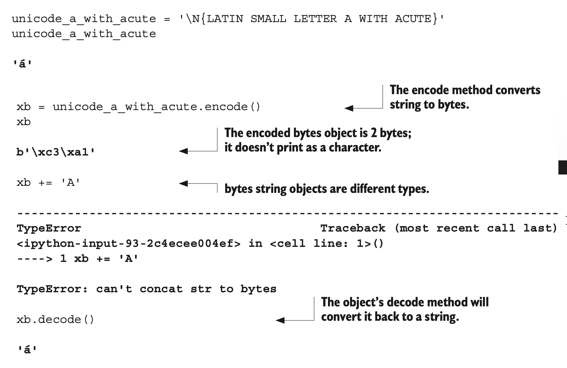
unicode_a ='\N{LATIN SMALL LETTER A}'# <-- Escapes by Unicode nameunicode_a#> 'a' # <-- ASCII characters are Unicode characters.unicode_a_with_acute ='\N{LATIN SMALL LETTER A WITH ACUTE}'unicode_a_with_acute#> 'á'"\u00E1"# <-- Escapes by number, using \u#> 'á'
This code shows how you can access characters, including common ASCII characters, by using their Unicode names with \N(Unicode name) or by using their number with \u.
6.3.3 Printing vs. evaluating strings with special characters
I talked earlier about the difference between evaluating a Python expression interactively and printing the result of the same expression by using the print function. Although the same string is involved, the two operations can produce screen outputs that look different. A string that’s evaluated at the top level of an interactive Python session is shown with all of its special characters as octal escape sequences, which makes clear what’s in the string. Meanwhile, the print function passes the string directly to the terminal program, which may interpret special characters in special ways. The following is what happens with a string consisting of an a followed by a newline, a tab, and a b:
'a\n\tb'#> 'a\n\tb'print('a\n\tb')#> a#> b
In the first case, the newline and tab are shown explicitly in the string; in the second, they’re used as newline and tab characters.
A normal print function also adds a newline to the end of the string. Sometimes (that is, when you have lines from files that already end with newlines), you may not want this behavior. Giving the print function an end parameter of “” causes the print function to suppress the final newline:
Most of the Python string methods are built into the standard Python string class, so all string objects have them automatically. The standard string module also contains some useful constants. Modules are discussed in detail in chapter 10.
For the purposes of this section, you need only remember that most string methods are attached to the string object they operate on by a dot (.), as in x.upper(). That is, they’re prepended with the string object followed by a dot. Because strings are immutable, the string methods are used only to obtain their return value and don’t modify the string object they’re attached to in any way.
I begin with those string operations that are the most useful and most commonly used; then I discuss some less commonly used but still useful operations. At the end of this section, I discuss a few miscellaneous points related to strings. Not all the string methods are documented here. See the documentation for a complete list of string methods.
6.4.1 The split and join string methods
Anyone who works with strings is almost certain to find the split and join methods invaluable. They’re the inverse of one another: split returns a list of substrings in the string, and join takes a list of strings and puts them together to form a single string with the original string between each element. Typically, split uses whitespace as the delimiter of the strings it’s splitting, but you can change that behavior via an optional argument.
String concatenation using + is useful but not efficient for joining large numbers of strings into a single string, because each time + is applied, a new string object is created. The previous Hello, World example produces three string objects, two of which are immediately discarded. A better option is to use the join function, which creates only one new string object:
The most common use of split is probably as a simple parsing mechanism for string-delimited records stored in text files. By default, split splits on any whitespace, not just a single space character, but you can also tell it to split on a particular sequence by passing it an optional argument:
x ="You\t\t can have tabs\t\n\t and newlines \n\n "\"mixed in"x.split()#> ['You', 'can', 'have', 'tabs', 'and', 'newlines', 'mixed', 'in']x ="Mississippi"x.split("ss")#> ['Mi', 'i', 'ippi']
Sometimes it’s useful to permit the last field in a joined string to contain arbitrary text, perhaps including substrings that may match what split splits on when reading in that data. You can do this by specifying how many splits split should perform when it’s generating its result, via an optional second argument. If you specify n splits, split goes along the input string until it has performed n splits (generating a list with n + 1 substrings as elements) or until it runs out of string. The following are some examples:
x ='a b c d'x.split(' ', 1)#> ['a', 'b c d']x.split(' ', 2)#> ['a', 'b', 'c d']x.split(' ', 9)#> ['a', 'b', 'c', 'd']
When using split with its optional second argument, you must supply a first argument. To get it to split on runs of whitespace while using the second argument, use None as the first argument.
예시
# 로그 형식: "날짜 시간 레벨 메시지"log_line ="2023-12-01 10:30:45 ERROR Failed to connect to server: Connection refused on port 8080"# 문제가 되는 방법 - 모든 공백으로 분할parts = log_line.split()print(parts)# ['2023-12-01', '10:30:45', 'ERROR', 'Failed', 'to', 'connect', 'to', 'server:', 'Connection', 'refused', 'on', 'port', '8080']# 메시지가 여러 조각으로 나뉘어짐!# 해결책 - maxsplit 사용parts = log_line.split(None, 3) # 최대 3번만 분할print(parts)# ['2023-12-01', '10:30:45', 'ERROR', 'Failed to connect to server: Connection refused on port 8080']date, time, level, message = partsprint(f"날짜: {date}")print(f"시간: {time}")print(f"레벨: {level}")print(f"메시지: {message}") # 전체 메시지가 보존됨
I use split and join extensively, usually when working with text files generated by other programs. If you want to create more standard output files from your programs, good choices are the csv and json modules in the Python standard library.
예시
# 1. 공백 정규화messy_text ="Hello world\t\tthis is\n\n messy"clean_text =' '.join(messy_text.split())print(clean_text) # "Hello world this is messy"# 2. 경로 처리unix_path ="/home/user/documents/file.txt"windows_path ='\\'.join(unix_path.split('/'))print(windows_path) # "\home\user\documents\file.txt"# 3. 데이터 변환pipe_delimited ="apple|banana|cherry|date"comma_delimited =','.join(pipe_delimited.split('|'))print(comma_delimited) # "apple,banana,cherry,date"# 4. 텍스트 필터링text_with_bad_words ="This is a good sentence. This is bad. This is okay."sentences = text_with_bad_words.split('. ')filtered ='. '.join([s for s in sentences if'bad'notin s])print(filtered) # "This is a good sentence. This is okay."
표준 출력 파일들
Prompt: csv, json을 포함해 현대적인 데이터 파일 형식에는 어떤 것이 있으며 그 특징을 예시와 함께 설명해주세요.
Quick check: split and join
How could you use split and join to change all the whitespace in string x to dashes, such as changing “this is a test” to “this-is-a-test”?
6.4.2 Converting strings to numbers
You can use the functions int and float to convert strings to integer or floating-point numbers, respectively. If they’re passed a string that can’t be interpreted as a number of the given type, these functions raise a ValueError exception. Exceptions are explained in chapter 14.
In addition, you may pass int an optional second argument, specifying the numeric base to use when interpreting the input string:
float('123.456')#> 123.456float('xxyy') #> ---------------------------------------------------------------------------#> ValueError Traceback (most recent call last)#> <ipython-input-30-14b25c5b2052> in <cell line: 1>()#> ----> 1 float('xxyy')#> ValueError: could not convert string to float: 'xxyy'int('3333')#> 3333int('123.456') # <-- Can't have decimal point in integer#> ---------------------------------------------------------------------------#> ValueError Traceback (most recent call last)#> <ipython-input-32-ed4c46a302ea> in <cell line: 1>()#> ----> 1 int('123.456')#> ValueError: invalid literal for int() with base 10: '123.456'int('10000', 8) # <-- Interprets 10000 as octal number#> 4096int('101', 2) # <-- Binary number#> 5int('ff', 16) # <-- Hexadecimal number255#> 255int('123456', 6) # <-- Can't interpret 123,456 as base 6 number#> ---------------------------------------------------------------------------#> ValueError Traceback (most recent call last)#> <ipython-input-36-bdc1281d81c5> in <cell line: 1>()#> ----> 1 int('123456', 6)#> ValueError: invalid literal for int() with base 6: '123456'
Did you catch the reason for that last error? I requested that the string be interpreted as a base 6 number, but the digit 6 can never appear in a base 6 number. Sneaky!
Quick check: Strings to numbers
Which of the following will not be converted to numbers, and why?
A trio of surprisingly useful simple methods are the strip, lstrip, and rstrip functions. strip returns a new string that’s the same as the original string, except that any whitespace at the beginning or end of the string has been removed. lstrip and rstrip work similarly, except that they remove whitespace only at the left or right end of the original string, respectively:
In this example, tab characters are considered to be whitespace. The exact meaning may differ across operating systems, but you can always find out what Python considers to be whitespace by accessing the string.whitespace constant. On my Windows system, Python returns the following:
The characters given in backslashed hex (\xnn) format represent the vertical tab and form-feed characters. The space character is in there as itself. It may be tempting to change the value of this variable, to attempt to affect how strip and so forth work, but don’t do it. Such an action isn’t guaranteed to give you the results you’re looking for.
You can, however, change which characters strip, rstrip, and lstrip remove by passing a string containing the characters to be removed as an extra parameter:
x ="www.python.org"x.strip("w") # <--Strips off all w's#> '.python.org'x.rstrip("gor") # <--Strips off all g's, o's, and r's from right side of string#> 'www.python.'x.strip(".gorw") # <--Strips off all dots, g's, o's, r's, and w's#> 'python'
Note that strip removes any and all of the characters in the extra parameter string, no matter in which order they occur.
The most common use for these functions is as a quick way to clean up strings that have just been read in. This technique is particularly helpful when you’re reading lines from files because Python always reads in an entire line, including the trailing newline, if one exists. When you get around to processing the line read in, you typically don’t want the trailing newline. rstrip is a convenient way to get rid of it.
There are also two new string methods to strip prefixes and suffixes:
x ="www.python.org"x.removeprefix("www.") # <-- Strips off only the prefix “www”#> 'python.org'x.removesuffix(".org") # <-- Strips off only the suffix “.org”#> 'www.python'
Unlike strip, removesuffix and removeprefix will only remove suffixes and prefixes that are exact matches for their parameters, which makes their behavior more predictable.
Quick check: strip
If the string x equals (name, date),\n, which of the following would return a string containing “name, date”?
x.rstrip("),")x.strip("),\n")x.strip("\n)(,")
6.4.4 String searching
The string objects provide several methods to perform simple string searches. Before I describe them, though, I’ll talk about another module in Python: re. (This module is discussed in depth in chapter 16.)
Another method for searching strings: The re module
The re module also does string searching but in a far more flexible manner, using regular expressions. Rather than search for a single specified substring, a re search can look for a string pattern. You could look for substrings that consist entirely of digits, for example.
Why am I mentioning this when re is discussed fully later? In my experience, many uses of basic string searches are inappropriate. You’d benefit from a more powerful searching mechanism but aren’t aware that one exists, so you don’t even look for something better. Perhaps you have an urgent project involving strings and don’t have time to read this entire book. If basic string searching does the job for you, that’s great. But be aware that you have a more powerful alternative.
The four basic string-searching methods are similar: find, rfind, index, and rindex. A related method, count, counts how many times a substring can be found in another string. I describe find in detail and then examine how the other methods differ from it.
find takes one required argument: the substring being searched for. find returns the position of the first character of the first instance of substring in the string object, or –1 if substring doesn’t occur in the string:
x ="Mississippi"x.find("ss")#> 2x.find("zz")#> -1
find can also take one or two additional, optional arguments. The first of these arguments, if present, is an integer start; it causes find to ignore all characters before position start in string when searching for substring. The second optional argument, if present, is an integer end; it causes find to ignore characters at or after position end in string:
x ="Mississippi"x.find("ss", 3)#> 5x.find("ss", 0, 3)#> -1
rfind is almost the same as find, except that it starts its search at the end of string and so returns the position of the first character of the last occurrence of substring in string:
x ="Mississippi"x.rfind("ss")#> 5
rfind can also take one or two optional arguments, with the same meanings as those for find.
index and rindex are identical to find and rfind, respectively, except for one difference: if index or rindex fails to find an occurrence of substring in string, it doesn’t return –1 but raises a ValueError exception. Exactly what this means will be clear after you read chapter 14.
count is used identically to any of the previous four functions but returns the number of nonoverlapping times the given substring occurs in the given string:
x ="Mississippi"x.count("ss")#> 2
You can use two other string methods to search strings: startswith and endswith. These methods return a True or False result, depending on whether the string they’re used on starts or ends with one of the strings given as parameters:
x ="Mississippi"x.startswith("Miss")#> Truex.startswith("Mist")#> Falsex.endswith("pi")#> Truex.endswith("p")#> False
Both startswith and endswith can look for more than one string at a time. If the parameter is a tuple of strings, both methods check for all the strings in the tuple and return True if any one of them is found:
x.endswith(("i", "u"))#> True
startswith and endswith are useful for simple searches where you’re sure that what you’re checking for is at the beginning or end of a line.
Quick check: String searching
If you wanted to check whether a line ends with the string “rejected”, what string method would you use? Would there be any other ways to get the same result?
6.4.5 Modifying strings
Strings are immutable, but string objects have several methods that can operate on a string and return a new string that’s a modified version of the original string. This provides much the same effect as direct modification, for most purposes. You can find a more complete description of these methods in the documentation.
You can use the replace method to replace occurrences of substring (its first argument) in the string with newstring (its second argument). This method also takes an optional third argument (see the documentation for details):
x ="Mississippi"x.replace("ss", "+++")#> 'Mi+++i+++ippi'
Like the string search functions, the re module is a much more powerful method of substring replacement.
The functions string.maketrans and string.translate may be used together to translate characters in strings into different characters. Although rarely used, these functions can simplify your life when they’re needed.
Suppose that you’re working on a program that translates string expressions from one computer language into another. The first language uses ~ to mean logical not, whereas the second language uses !; the first language uses ^ to mean logical, and the second language uses &; the first language uses ( and ), whereas the second language uses [ and ]. In a given string expression, you need to change all instances of ~ to !, all instances of ^ to &, and all instances of ( to [, and all instances of ) to ]. You could do this by using multiple invocations of replace, but an easier and more efficient way is
The second line uses maketrans to make up a translation table from its two string arguments. The two arguments must each contain the same number of characters, and a table is made such that looking up the nth character of the first argument in that table gives back the nth character of the second argument.
Next, the table produced by maketrans is passed to translate. Then translate goes over each of the characters in its string object and checks to see whether they can be found in the table given as the second argument. If a character can be found in the translation table, translate replaces that character with the corresponding character looked up in the table to produce the translated string.
You can also use translate with an optional argument to specify characters that should be removed from the string. To remove characters, you would use empty strings for the first and second arguments and include a third string of characters to remove:
x ="~x ^ (y % z)"table = x.maketrans("", "", "()~^%")x.translate(table)#> 'x y z'
Here all of the punctuation marks in the original string are in the third parameter, a string containing the characters to remove.
Other functions in the string module perform more specialized tasks. string .lower converts all alphabetic characters in a string to lowercase, and upper does the opposite. capitalize capitalizes the first character of a string, and title capitalizes all words in a string. swapcase converts lowercase characters to uppercase and uppercase to lowercase in the same string. expandtabs gets rid of tab characters in a string by replacing each tab with a specified number of spaces. ljust, rjust, and center pad a string with spaces to justify it in a certain field width. zfill left-pads a numeric string with zeros. Refer to the documentation for details on these methods.
6.4.6 Modifying strings with list manipulations
Because strings are immutable objects, you have no way to manipulate them directly in the same way that you can manipulate lists. Although the operations that produce new strings (leaving the original strings unchanged) can be useful, sometimes you want to be able to manipulate a string as though it were a list of characters. In that case, turn the string into a list of characters, do whatever you want, and then turn the resulting list back into a string:
text ="Hello, World"wordList =list(text)wordList[6:] = [] # <-- Removes everything after commawordList.reverse()text ="".join(wordList) # <-- Joins with no space betweenprint(text)#> ,olleH
You can also turn a string into a tuple of characters by using the built-in tuple function. To turn the list back into a string, use ““.join().
You shouldn’t go overboard with this method because it causes the creation and destruction of new string objects, which is relatively expensive. Processing hundreds or thousands of strings in this manner probably won’t have much of an impact on your program; processing millions of strings probably will.
Quick check: Modifying strings
What would be a quick way to change all punctuation in a string to spaces?
6.4.7 Useful methods and constants
string objects also have several useful methods to report various characteristics of the string, such as whether it consists of digits or alphabetic characters or is all uppercase or lowercase:
x ="123"x.isdigit()#> Truex.isalpha()#> Falsex ="M"x.islower()#> Falsex.isupper()#> True
For a list of all the possible string methods, refer to the string section of the official Python documentation.
Finally, the string module defines some useful constants. You’ve already seen string.whitespace, which is a string made up of the characters Python thinks of as whitespace on your system. string.digits is the string ‘0123456789’. string .hexdigits includes all the characters in string.digits, as well as ‘abcdefABCDEF’, the extra characters used in hexadecimal numbers. string.octdigits contains ‘01234567’—only those digits used in octal numbers. string.ascii_lowercase contains all lowercase ASCII alphabetic characters; string.ascii_uppercase contains all ASCII uppercase alphabetic characters; string.ascii_letters contains all the characters in string.ascii_lowercase and string.ascii_uppercase. You might be tempted to try assigning to these constants to change the behavior of the language. Python would let you get away with this action, but it probably would be a bad idea.
Remember that strings are sequences of characters, so you can use the convenient Python in operator to test for a character’s membership in any of these strings, although usually the existing string methods are simpler and easier. The most common string operations are shown in table 6.2.
Table 6.2 Common string operations
String operation
Explanation
Example
+
Adds two strings together
x = "hello " + "world"
*
Replicates a string
x = " " * 20
upper
Converts a string to uppercase
x.upper()
lower
Converts a string to lowercase
x.lower()
title
Capitalizes the first letter of each word in a string
x.title()
find, index
Searches for the target in a string
x.find(y) x.index(y)
rfind, rindex
Searches for the target in a string from the end of the string
x.rfind(y) x.rindex(y)
startswith, endswith
Checks the beginning or end of a string for a match
x.startswith(y) x.endswith(y)
replace
Replaces the target with a new string
x.replace(y, z)
strip, rstrip, lstrip
Removes whitespace or other characters from the ends of a string
x.strip()
encode
Converts a Unicode string to a bytes object
x.encode("utf_8")
Note that these methods don’t change the string itself; they return either a location in the string or a string.
Try this: String operations
Suppose that you have a list of strings in which some (but not necessarily all) of the strings begin and end with the double-quote character:
x = ['"abc"', 'def', '"ghi"', '"klm"', 'nop']
What code would you use on each element to remove just the double quotes?
What code could you use to find the position of the last p in Mississippi? When you’ve found that position, what code would you use to remove just that letter?
6.5 Converting objects to strings
In Python, almost anything can be converted to some sort of a string representation by using the built-in repr function. Lists are the only complex Python data types you’re familiar with so far, so here, I turn some lists into their representations:
repr([1, 2, 3])#> '[1, 2, 3]'x = [1]x.append(2)x.append([3, 4])'the list x is '+repr(x)#> 'the list x is [1, 2, [3, 4]]'
The example uses repr to convert the list x to a string representation, which is then concatenated with the other string to form the final string. Without the use of repr, this code wouldn’t work. In an expression like “string” + [1, 2] + 3, are you trying to add strings, add lists, or just add numbers? Python doesn’t know what you want in such a circumstance, so it does the safe thing (raises an error) rather than make any assumptions. In the previous example, all the elements had to be converted to string representations before the string concatenation would work.
Lists are the only complex Python objects that I’ve described to this point, but repr can be used to obtain some sort of string representation for almost any Python object. To see this, try repr around a built-in complex object, which is an actual Python function:
repr(len)#> '<built-in function len>'
Python hasn’t produced a string containing the code that implements the len function, but it has at least returned a string——that describes what that function is. If you keep the repr function in mind and try it on each Python data type (dictionaries, tuples, classes, and the like) in the book, you’ll see that no matter what type of Python object you have, you can get a string that describes something about that object.
This is great for debugging programs. If you’re in doubt about what’s held in a variable at a certain point in your program, use repr and print out the contents of that variable.
I’ve covered how Python can convert any object to a string that describes that object. The truth is, Python can do this in either of two ways. The repr function always returns what might be loosely called the formal string representation of a Python object. More specifically, for simpler objects repr returns a string representation of a Python object from which the original object can be rebuilt. For large, complex objects, this may not be the sort of thing you want to see, so repr returns some descriptive text.
Python also provides the built-in str function. In contrast to repr, str is intended to produce printable string representations, and it can be applied to any Python object. str returns what might be called the informal string representation of the object. A string returned by str need not define an object fully and is intended to be read by humans, not by Python code.
You won’t notice any difference between repr and str when you start using them, because until you begin using the object-oriented features of Python, there’s no difference. str applied to any built-in Python object always calls repr to calculate its result. Only when you start defining your own classes does the difference between str and repr become important, as discussed in chapter 15.
So why talk about this now? I want you to be aware that there’s more going on behind the scenes with repr than just being able to easily write print functions for debugging. As a matter of good style, you may want to get into the habit of using str rather than repr when creating strings for displaying information.
6.6 Using the format method
You can format strings in Python 3 in three ways. One way is to use the string class’s format method. The format method combines a format string containing replacement fields marked with { }, with replacement values taken from the parameters given to the format command. If you need to include a literal { or } in the string, you double it to {{ or }}. The format command is a powerful string-formatting mini-language that offers almost endless possibilities for manipulating string formatting. Conversely, it’s fairly simple to use for the most common use cases, so I look at a few basic patterns in this section. Then, if you need to use the more advanced options, you can refer to the string-formatting section of the standard library documentation.
6.6.1 The format method and positional parameters
A simple way to use the string format method is with numbered replacement fields that correspond to the parameters passed to the format function:
"{0} is the {1} of {2}".format("Ambrosia", "food", "the gods") #> 'Ambrosia is the food of the gods'"{{Ambrosia}} is the {0} of {1}".format("food", "the gods") #> '{Ambrosia} is the food of the gods'
Note that the format method is applied to the format string, which can also be a string variable. Doubling the { } characters escapes them so that they don’t mark a replacement field.
This example has three replacement fields, {0}, {1}, and {2}, which are in turn filled by the first, second, and third parameters. No matter where in the format string you place {0}, it’s always replaced by the first parameter, and so on.
You can also use named parameters.
6.6.2 The format method and named parameters
The format method also recognizes named parameters and replacement fields:
"{food} is the food of {user}".format(food="Ambrosia", user="the gods")#> 'Ambrosia is the food of the gods'
In this case, the replacement parameter is chosen by matching the name of the replacement field with the name of the parameter given to the format command.
You can also use both positional and named parameters, and you can even access attributes and elements within those parameters:
"{0} is the food of {user[1]}".format("Ambrosia", user=["men", "the gods", "others"])#> 'Ambrosia is the food of the gods'
In this case, the first parameter is positional, and the second, user[1], refers to the second element of the named parameter user.
6.6.3 Format specifiers
Format specifiers let you specify the result of the formatting with even more power and control than the formatting sequences of the older style of string formatting. The format specifier lets you control the fill character, alignment, sign, width, precision, and type of the data when it’s substituted for the replacement field. As noted earlier, the syntax of format specifiers is a mini-language in its own right and too complex to cover completely here, but the following examples give you an idea of its usefulness:
print("{0:10} is the food of gods".format("Ambrosia"))print("{0:{1}} is the food of gods".format("Ambrosia", 10))print("{food:{width}} is the food of gods".format(food="Ambrosia", width=10))print("{0:>10} is the food of gods".format("Ambrosia"))print("{0:&>10} is the food of gods".format("Ambrosia"))
Ambrosia   is the food of gods
Ambrosia   is the food of gods
Ambrosia   is the food of gods
  Ambrosia is the food of gods
&&Ambrosia is the food of gods
:10 is a format specifier that makes the field 10 spaces wide and pads with spaces. :{1} takes the width from the second parameter. :>10 forces right justification of the field and pads with spaces. :&>10 forces right justification and pads with & instead of spaces.
Quick check: The format() method
What will be in x when the following snippets of code are executed?
Starting in Python 3.6, the newest way to create strings is called f-strings. F-strings, as they’re commonly called because they are prefixed with f, are a way to include the values of arbitrary Python expressions inside literal strings. They use curly braces (“{ }”) to include and evaluate Python expressions. The syntax of f-strings is almost identical to that of the format method, but without an explicit call to format() they are more compact and easier to read. Thanks to their simplicity, they have become very common.
To use an f-string, you simply put an “f” right before the first quote and then include the Python expressions you want interpolated into the string in curly braces. The following examples give you a basic idea of how f-strings work:
value =42message =f"The answer is {value}"print(message)#> The answer is 42primes = [1, 2, 3, 5]f"sum of first 4 primes is {sum(primes)}"#> 'sum of first 4 primes is 11'
Just as with the format method, format specifiers may be added:
PI =3.1415print(f"PI is {PI:{10}.{2}}")#> PI is 3.1
Another useful feature of f-strings is that adding an “=” after an expression in curly braces will give you “debugging” output by showing both the expression and its value:
print(f"{PI=:{10}.{2}}")#> PI= 3.1primes = [1, 2, 3, 5]f"sum of first 4 primes is {sum(primes)=}"#> 'sum of first 4 primes is sum(primes)=11'
All of the format specifiers that work for the format method described here should also work for f-strings. While f-strings were a bit limited in their early versions, they have proved so useful as a concise and readable way of creating strings with the values of variables and expressions that they have been extended and are currently used extensively.
예시
x ="Ambrosia"print(f"{x:=>12} is the food of gods")#> ====Ambrosia is the food of godsPI =3.1415print(f"PI is {PI:.2}.")print(f"PI is {PI:.2g}.")print(f"PI is {PI:.2f}.")print(f"PI is {PI:.2e}.")#> PI is 3.1.#> PI is 3.1.#> PI is 3.14.#> PI is 3.14e+00.rate =0.0325print(f"rate is {rate:.2%}")#> rate is 3.25%price =123456print(f"price is ₩{price:,}") # unicode 표현: print(f"price is \u20A9{price:,}")print(f"price is {price:10,} KRW")print(f"price is {price:10,.0f} KRW")#> price is ₩123,456#> price is 123,456 KRW#> price is 123,456 KRW
6.8 Formatting strings with %
This section covers formatting strings with the string modulus (%) operator. This operator is used to combine Python values into formatted strings for printing or other use. C users will notice a strange similarity to the printf family of functions. The use of % for string formatting is the old style of string formatting, and I cover it here because it was the standard in earlier versions of Python, and you’re likely to see it in code that’s been ported from earlier versions of Python or was written by coders who are familiar with those versions. This style of formatting shouldn’t be used in new code, however, because it’s slated to be deprecated and then removed from the language in the future.
The following is an example:
"%s is the %s of %s"% ("Ambrosia", "food", "the gods")#> 'Ambrosia is the food of the gods'
The string modulus operator (the last % that occurs in the line, not the three instances of %s that come before it in the example) takes two parts: the left side, which is a string, and the right side, which is a tuple. The string modulus operator scans the left string for special formatting sequences and produces a new string by substituting the values on the right side for those formatting sequences, in order. In this example, the only formatting sequences on the left side are the three instances of %s, which stands for “Stick a string in here.”
Passing in different values on the right side produces different strings:
"%s is the %s of %s"% ("Nectar", "drink", "gods")#> 'Nectar is the drink of gods'"%s is the %s of the %s"% ("Brussels Sprouts", "food", "foolish")#> 'Brussels Sprouts is the food of the foolish'
The members of the tuple on the right have str applied to them automatically by %s, so they don’t have to already be strings:
x = [1, 2, "three"]"The %s contains: %s"% ("list", x)#> 'The list contains: [1, 2, 'three']'
6.8.1 Using formatting sequences
All formatting sequences are substrings contained in the string on the left side of the central %. Each formatting sequence begins with a percent sign and is followed by one or more characters that specify what is to be substituted for the formatting sequence and how the substitution is to be accomplished. The %s formatting sequence used previously is the simplest formatting sequence; it indicates that the corresponding string from the tuple on the right side of the central % should be substituted in place of the %s.
Other formatting sequences can be more complex. The following sequence specifies the field width (total number of characters) of a printed number to be 6, specifies the number of characters after the decimal point to be 2, and left-justifies the number in its field. I’ve put this formatting sequence in angle brackets so you can see where extra spaces are inserted into the formatted string:
"Pi is <%-6.2f>"%3.14159# use of the formatting sequence: %–6.2f#> 'Pi is <3.14 >'
All the options for characters that are allowable in formatting sequences are given in the documentation. There are quite a few options, but none is particularly difficult to use. Remember that you can always try a formatting sequence interactively in Python to see whether it does what you expect it to do.
6.8.2 Named parameters and formatting sequences
Finally, one additional feature available with the % operator can be useful in certain circumstances. Unfortunately, to describe it, I have to employ a Python feature that I haven’t yet discussed in detail: dictionaries, commonly called hash tables or associative arrays in other languages. You can skip ahead to chapter 7 to learn about dictionaries; skip this section for now and come back to it later; or read straight through, trusting the examples to make things clear.
Formatting sequences can specify what should be substituted for them by name rather than by position. When you do this, each formatting sequence has a name in parentheses immediately following the initial % of the formatting sequence, like so:
"%(pi).2f"# <-- 'Note the name in parentheses.'
In addition, the argument to the right of the % operator is no longer given as a single value or tuple of values to be printed but as a dictionary of values to be printed, with each named formatting sequence having a correspondingly named key in the dictionary. Using the previous formatting sequence with the string modulus operator, you might produce code like the following:
This code is particularly useful when you’re using format strings that perform a large number of substitutions, because you no longer have to keep track of the positional correspondences of the right-side tuple of elements with the formatting sequences in the format string. The order in which elements are defined in the dict argument is irrelevant, and the template string may use values from dict more than once (as it does with the pi entry).
Controlling output with the print function
Python’s built-in print function also has some options that can make handling simple string output easier. When used with one parameter, print prints the value and a newline character, so that a series of calls to print prints each value on a separate line:
print("a")print("b")#> a#> b
But print can do more. You can also give the print function several arguments, and those arguments are printed on the same line, separated by spaces and ending with a newline:
print("a", "b", "c")#> a b c
If that’s not quite what you need, you can give the print function additional parameters to control what separates each item and what ends the line:
print("a", "b", "c", sep="|")#> a|b|cprint("a", "b", "c", end="\n\n")#> a b c#>
Finally, the print function can be used to print to files as well as console output:
Using the print function’s options gives you enough control for simple text output, but more complex situations are best served by using the format method.
Quick check: Formatting strings with %
What would be in the variable x after the following snippets of code have executed?
x ="%.2f"%1.1111x ="%(a).2f"% {'a':1.1111}x ="%(a).08f"% {'a':1.1111}
6.9 Bytes
A bytes object is similar to a string object but with an important difference: A string is an immutable sequence of Unicode characters, whereas a bytes object is a sequence of integers with values from 0 to 256. Bytes can be necessary when you’re dealing with binary data, such as reading from a binary data file.
The key thing to remember is that bytes objects may look like strings, but they can’t be used exactly like strings or combined with strings:
The first thing you can see is that to convert from a regular (Unicode) string to bytes, you need to call the string’s encode method. After it’s encoded to a bytes object, the character is 2 bytes and no longer prints the same way that the string did. Further, if you attempt to add a bytes object and a string object together, you get a type error because the two types are incompatible. Finally, to convert a bytes object back to a string, you need to call that object’s decode method.
Most of the time, you shouldn’t need to think about Unicode or bytes at all. But when you need to deal with international character sets (an increasingly common problem), you must understand the difference between regular strings and bytes.
Quick check: Bytes
For which of the following kinds of data would you want to use a string? For which could you use bytes?
Data file storing binary data
Text in a language with accented characters
Text with only uppercase and lowercase roman characters
결과
11101010 10110000 10000000 = 0xEA 0xB0 0x80
= b'\xea\xb0\x80'
6.10 Preprocessing text
In processing raw text, it’s quite often necessary to clean and normalize the text before doing anything else. If you want to find the frequency of words in text, for example, you can make the job easier if, before you start counting, you make sure that everything is lowercase (or uppercase, if you prefer) and that all punctuation has been removed. You can also make things easier by breaking the text into a series of words. In this lab, the task is to read the first part of the first chapter of Moby Dick, make sure that everything is one case, remove all punctuation, and write the words one per line to a second file. As mentioned in the previous chapter, you should attempt to create a solution on your own before using AI to generate one.
To solve the problem, your code will need to open the source file, moby_01.txt. If you are using the Jupyter notebook, you can just execute the cell right before the lab. You can also download the file from the GitHub repository’s folder for this chapter and save it in the directory you are working in.
You will also need to perform the operations to clean the text: making everything lowercase, removing punctuation, splitting the text into words, and writing the cleaned output to a file. My suggestion is that you process the file line by line since that will save memory, and it’s easy to read and write line by line in Python.
Because I haven’t yet covered reading and writing files, I provide the code for those operations—just put your code in place of the comments in the for loop:
# Download the filewget https://raw.githubusercontent.com/nceder/qpb4e/main/code/Chapter%2006/moby_01.txt # 또는 curl 명령어 사용curl-O https://raw.githubusercontent.com/nceder/qpb4e/main/code/Chapter%2006/moby_01.txt
withopen("moby_01.txt") as infile:withopen("moby_01_clean.txt", "w") as outfile:for line in infile:# make all one (lower) case# remove punctuation# split into words# write all words for line outfile.write(cleaned_words)
Hint: You can work on one cleaning step at a time. First, create the code to make everything lowercase, and check to see that the text in the output file is lowercase. Then, work on removing the punctuation, and make sure that works, and so on.
6.10.1 Solving the problem with AI-generated code
Using AI to generate code for this problem is fairly simple. In this case, it’s probably easier to let the AI tool take care of opening, reading, and writing the files. To create a prompt, we need to be sure to include requirements:
Open the file moby_01.txt.
Read the lines of text.
Make all the text lowercase.
Remove any punctuation.
Split the line into words.
Write the words of the line to a file moby_01_clean.text.
If you want to try generating a solution using AI, go ahead and create a prompt and see what you get, and test to see if that code works correctly.
6.10.2 Solutions and discussion
Unsurprisingly, my solution and the AI solution were very similar. As we will see, however, the AI version misses a couple of tricks that would slightly improve efficiency.
The human solution
Solving this problem using the framework provided here is fairly straightforward—just take it one step at a time:
# Solution created by the authorimport stringpunct =str.maketrans("", "", string.punctuation)withopen("moby_01.txt") as infile:withopen("moby_01_clean.txt", "w") as outfile:for line in infile:# make all one case cleaned_line = line.lower()# remove punctuation cleaned_line = cleaned_line.translate(punct)# split into words words = cleaned_line.split() cleaned_words ="\n".join(words) +"\n"# write all words for line outfile.write(cleaned_words)
This solution is concise and reasonably efficient. In it we import the string library so that we can create a translation table to remove punctuation using Python’s list of punctuation rather than creating our own. In processing a line of text, we first use the lower() method on the entire line, and then use the translate method on the entire line. We then split the line into words, which will return a list of the words without any whitespace, and finally rejoin the words with a newline, which means that when written to the file, there will be one word per line.
The AI version
Creating the AI version is a bit simpler in that we don’t need to keep the scaffolding for opening, reading, and writing files, since the code generator should know how to do that. A reasonably concise prompt for what we need would be
For every line the file moby_01.txt, make everything lower case, remove
punctuation, and split into words. Write the words one per line to the file
moby_01_clean.txt.
For this problem, the solutions generated in Colaboratory and in Copilot were very similar. A good representative is the following solution generated by Copilot:
import string# Open the input file for readingwithopen('moby_01.txt', 'r') as input_file:# Open the output file for writingwithopen('moby_01_clean.txt', 'w') as output_file:# Iterate over each line in the input filefor line in input_file:# Convert the line to lowercase line = line.lower()# Remove punctuation from the line line = line.translate(str.maketrans('', '', string.punctuation)) # <-- Creates a new translation table for every line# Split the line into words words = line.split()# Write each word to the output filefor word in words: output_file.write(word +'\n')
The solution is nicely formatted and well commented, although I might say that a comment like # Iterate over each line in the input file is obvious and redundant coming right before the line for line in input_file:, but that’s not important.
A more serious problem is the way that the code uses the translate method. Note that instead of creating a translation table for punctuation once at the beginning of the program (as the human-created version does), it creates a new translation table on the fly for every line. Experienced coders will cringe—repeating an operation inside a loop unnecessarily can make your code run much, much slower and is the sort of rookie mistake most coders want to avoid.
One solution offered by Colaboratory makes this problem even worse. Instead of using the translate method, it suggests looping over every character in string .punctuation using the replace method to remove it from the string:
# Remove punctuationfor char in string.punctuation: line = line.replace(char, '')
Here again we have a loop where translate is a single operation, and in this case, we are looping over all of the punctuation characters in every line and creating a new string object every time a punctuation character is found and removed. While this isn’t a problem with a relatively small file, it can quickly become a big problem if we have to process a dataset with millions of lines.
A similar problem occurs in the last section, which writes the words to the output file. While not as much of a potential performance problem as the first one, it’s still a problem, for two reasons. First, it loops over the list of words in the line, and second, it uses string concatenation (+) to add the newlines. While Python for loops are heavily optimized, using a loop when one isn’t needed will still make things slower than they have to be, and using the + to add two strings together forces the creation of a new string, which also takes a bit of time.
The human version gets around this by using the join method with a newline character. Instead of a loop, this is a single operation, and instead of creating a new string object for every word, it creates just one for the entire line.
In this lab, the code generated by AI tools does the job, but if you tried to put that code into production under any sort of load, the slow performance might well become a problem.
Summary
Python strings have powerful text-processing features, including searching and replacing, trimming characters, and changing case.
Strings are immutable; they can’t be changed in place.
Operations that appear to change strings actually return a copy with the changes.
There are three ways to combine strings and the values of Python expressions: the format method, f-strings, and the legacy method using %.
The format method has an extensive formatting language to control its output.
F-strings are a very convenient way to create strings containing the values of variables and expressions and are now used widely.
Python has a bytes data type that contains ints in the range 0 to 255; they look similar to strings but need to be decoded to be converted to strings.
7. Dictionaries
This chapter covers
Defining a dictionary
Using dictionary operations
Determining what can be used as a key
Creating sparse matrices
Using dictionaries as caches
Trusting the efficiency of dictionaries
This chapter discusses dictionaries, Python’s name for associative arrays or maps, which it implements by using hash tables. Dictionaries are amazingly useful, even in simple programs.
Because dictionaries are less familiar to many programmers than other basic data structures such as lists and strings, some of the examples illustrating dictionary use are slightly more complex than the corresponding examples for other built-in data structures. It may be necessary to read parts of chapter 8 to fully understand some of the examples in this chapter.
7.1 What is a dictionary?
If you’ve never used associative arrays or hash tables in other languages, a good way to start understanding the use of dictionaries is to compare them with lists:
Values in lists are accessed by means of integers called indices, which indicate where in the list a given value is found.
Dictionaries access values by means of integers, strings, or other Python objects called keys, which indicate where in the dictionary a given value is found. In other words, both lists and dictionaries provide indexed access to arbitrary values, but the set of items that can be used as dictionary indices is much larger than, and contains, the set of items that can be used as list indices. Also, the mechanism that dictionaries use to provide indexed access is quite different from that used by lists.
Both lists and dictionaries can store objects of any type.
Values stored in a list are implicitly ordered by their positions in the list, because the indices that access these values are consecutive integers. You may or may not care about this ordering, but you can use it if desired. Values stored in a dictionary are not implicitly ordered relative to one another because dictionary keys aren’t just numbers.
If you’re using a dictionary but also care about the order of the items (the order in which they were added, that is), since Python 3.6 dictionaries store their items in the order they were added. There is also an ordered dictionary, which is a dictionary subclass that can be imported from the collections module and which offers a few extra features, such as a move_to_end method and the ability to access items in reverse order. You can also define an order on the items in a dictionary by using another data structure (often a list) to store such an ordering explicitly.
In spite of the differences between them, the use of dictionaries and lists often appears to be the same. As a start, an empty dictionary is created much like an empty list but with curly braces instead of square brackets:
x_list = [] # <--- A listy_dic = {} # <--- A dictionary
Here, the first line creates a new, empty list and assigns the variable x to it. The second line creates a new, empty dictionary and assigns the variable y to it.
After you create a dictionary, you may store values in it as though it were a list:
y_dic[0] ='Hello'y_dic[1] ='Goodbye'
Even in these assignments, there’s already a significant operational difference between the dictionary and list usage. Trying to do the same thing with a list would result in an error, because in Python, it’s illegal to assign to a position in a list that doesn’t exist. For example, if you try to assign to the 0th element of the list x, you receive an error:
x_list[0] ='Hello'# ---------------------------------------------------------------------------# IndexError Traceback (most recent call last)# <ipython-input-1-ba4ef4c8f6ab> in <cell line: 3>()# 1 x_list = []# 2 y_dic = {}# ----> 3 x_list[0] = 'Hello'# IndexError: list assignment index out of range
This is not a problem to dictionaries; new positions in dictionaries are created as necessary.
Having stored some values in the dictionary, now you can access and use them:
Overall, this makes a dictionary look pretty much like a list. Now for the big difference: you can store (and use) values under keys that aren’t integers:
This is definitely something that can’t be done with lists! Whereas list indices must be integers, dictionary keys are much less restricted; they may be numbers, strings, or one of a wide range of other Python objects. This makes dictionaries a natural for jobs that lists can’t do. For example, it makes more sense to implement a telephone directory application with dictionaries than with lists because the phone number for a person can be stored and indexed by that person’s last name.
A dictionary is a way of mapping from one set of arbitrary objects to an associated but equally arbitrary set of objects. Actual dictionaries, thesauri, or translation books are good analogies in the real world. To see how natural this correspondence is, here’s the start of an English-to-French color translator:
english_to_french = {} # <-- Creates empty dictionaryenglish_to_french['red'] ='rouge'# <-- Stores three words in itenglish_to_french['blue'] ='bleu'english_to_french['green'] ='vert'print("red is", english_to_french['red']) # <--- Obtains value for "red"#> red is rouge
Try this: Create a dictionary
Write the code to ask a user for three names and three ages. After the names and ages are entered, ask the user for one of the names, and print the correct age.
Show the code
name_age = {}for i inrange(3): name =input("Name? ") age =int(input("Age? ")) name_age[name] = agename_choice =input("Name to find? ")print(name_age[name_choice])
7.2 Other dictionary operations
Besides basic element assignment and access, dictionaries support several operations. You can define a dictionary explicitly as a series of key-value pairs separated by commas:
english_to_french = {'red': 'rouge', 'blue': 'bleu', 'green': 'vert'}# len returns the number of entries in a dictionary: len(english_to_french)#> 3
You can obtain all the keys in the dictionary with the keys method. This method is often used to iterate over the contents of a dictionary using Python’s for loop, described in chapter 8:
In Python 3.5 and earlier, the order of the keys in a list returned by keys has no meaning; the keys aren’t necessarily sorted, and they don’t necessarily occur in the order in which they were created. Your Python code may print out the keys in a different order than my Python code did. If you need keys sorted, you can store them in a list variable and then sort that list. However, as mentioned earlier, starting with Python 3.6, dictionaries preserve the order that the keys were created and return them in that order.
It’s also possible to obtain all the values stored in a dictionary by using values:
Like keys, this method is often used in conjunction with a for loop to iterate over the contents of a dictionary.
예제
# for 루프로 키 출력for key in english_to_french:print(key)#> red#> blue#> green# for 루프로 키 출력for key in english_to_french.keys():print(key)#> red#> blue#> green# for 루프로 키-값 쌍 출력for english, french in english_to_french.items():print(f"{english} is {french} in French")#> red is rouge in French#> blue is bleu in French#> green is vert in French
The del statement can be used to remove an entry (key-value pair) from a dictionary:
The keys, values, and items methods return not lists but views that behave like sequences but are dynamically updated whenever the dictionary changes. That’s why you need to use the list function to make them appear as a list in these examples. Otherwise, they behave like sequences, allowing code to iterate over them in a for loop, using in to check membership in them, and so on.
The view returned by keys (and in some cases the view returned by items) also behaves like a set, with union, difference, and intersection operations.
Dictionary View Objects 설명
딕셔너리는 세 개의 뷰 객체를 반환: keys, values, items(튜플 형태)
동적 업데이트
student_scores = {'Alice': 85, 'Bob': 90, 'Charlie': 78}keys_view = student_scores.keys() # 리스트가 아닌 View 객체student_scores['Diana'] =98# 딕셔너리 수정 (새로운 키 추가)# keys_view가 자동으로 업데이트됨! (새로운 호출 없이)keys_view#> dict_keys(['Alice', 'Bob', 'Charlie', 'Diana'])
# 어제 재고: {상품명: 가격}stock_yesterday = {"사과": 1500,"바나나": 3000,"포도": 5000,"수박": 20000,}# 오늘 재고: {상품명: 가격}stock_today = {"사과": 1500, # 가격 변동 없음"바나나": 3200, # 가격 인상"딸기": 8000, # 신규 입고"수박": 20000, # 가격 변동 없음}# 1. 품절된 상품 찾기 (어제 keys - 오늘 keys)# set의 차집합(difference) 연산 사용sold_out = stock_yesterday.keys() - stock_today.keys()# 2. 신규 입고 상품 찾기 (오늘 keys - 어제 keys)new_items = stock_today.keys() - stock_yesterday.keys()ic(new_items) # ic| new_items: {'딸기'}# 3. 가격이 변경된 상품 찾기# 어제와 오늘 모두 판매 중인 상품 목록 (교집합, intersection)common_items = stock_yesterday.keys() & stock_today.keys()ic(common_items) # ic| common_items: {'바나나', '사과', '수박'}
중요:values() view는 set 연산을 지원하지 않음 (값은 중복될 수 있고 hashable하지 않을 수 있기 때문).
Attempting to access a key that isn’t in a dictionary is an error in Python. To handle this error, you can test the dictionary for the presence of a key with the in keyword, which returns True if a dictionary has a value stored under the given key and False otherwise:
Alternatively, you can use the get function. This function returns the value associated with a key if the dictionary contains that key but returns its second argument if the dictionary doesn’t contain the key:
print(english_to_french.get('blue', 'No translation'))#> bleuprint(english_to_french.get('chartreuse', 'No translation')) # <-- Chartreuse not found, "No translation" is returned.#> No translation
The second argument is optional. If that argument isn’t included, get returns None if the dictionary doesn’t contain the key.
Similarly, if you want to safely get a key’s value and make sure that it’s set to a default in the dictionary, you can use the setdefault method:
print(english_to_french.setdefault('chartreuse', 'No translation')) # <--- Chartreuse not found and is added as key, and "No translation" is returned and added as its value.#> No translation
The difference between get and setdefault is that after the setdefault call, there’s a key in the dictionary ‘chartreuse’ with the value ‘No translation’.
There is also a defaultdict subclass of dict that you can import from the collections module, and instances of defaultdict can be given a default value and will automatically work the same was as setdefault.
예제
from collections import defaultdict# Create a defaultdict with 'No translation' as the default valuefrench_dict = defaultdict(lambda: 'No translation')french_dict['red'] ='rouge'french_dict['blue'] ='bleu'print(french_dict['red']) # Returns existing value#> rougeprint(french_dict['chartreuse']) # Returns default value and adds the key#> No translationprint(french_dict) # 'chartreuse' is now in the dictionary#> defaultdict(<function <lambda> at ...>, {'red': 'rouge', 'blue': 'bleu', 'chartreuse': 'No translation'})
defaultdict(int): 존재하지 않는 키에 접근하면 기본값으로 정수 0을 생성함. 아이템 개수를 셀 때 유용
counts = {}for fruit in ['apple', 'orange', 'apple']: counts.setdefault(fruit, 0) # 매번 setdefault 메서드를 호출하고 키 존재 여부를 확인하는 과정을 거침 counts[fruit] +=1print(counts)# > {'apple': 2, 'orange': 1}
You can obtain a copy of a dictionary by using the copy method:
This method makes a shallow copy of the dictionary, which is likely to be all you need in most situations. For dictionaries that contain any modifiable objects as values (for example, lists or other dictionaries), you may want to make a deep copy by using the copy.deepcopy function. See chapter 5 for an introduction to the concept of shallow and deep copies.
The update method updates the dictionary it is a member of with all the key-value pairs of a second dictionary. For keys that are common to both dictionaries, the values from the second dictionary override those of the first:
Dictionary methods give you a full set of tools to manipulate and use dictionaries. For quick reference, table 7.1 lists some of the main dictionary functions.
Table 7.1 Dictionary operations
Dictionary operation
Explanation
Example
{}
Creates an empty dictionary
x = {}
len
Returns the number of entries in a dictionary
len(x)
keys
Returns a view of all keys in a dictionary
x.keys()
values
Returns a view of all values in a dictionary
x.values()
items
Returns a view of all items in a dictionary
x.items()
del
Removes an entry from a dictionary
del(x[key])
in
Tests whether a key exists in a dictionary
'y' in x
get
Returns the value of a key or a configurable default
x.get('y', None)
setdefault
Returns the value if the key is in the dictionary; otherwise, sets the value for the key to the default and returns the value
x.setdefault('y', None)
copy
Makes a shallow copy of a dictionary
y = x.copy()
update
Combines the entries of two dictionaries
x.update(z)
This table isn’t a complete list of all dictionary operations. For a complete list, refer to the Python standard library documentation.
Quick check: Dictionary operations
Assume that you have a dictionary x = {‘a’:1, ‘b’:2, ‘c’:3, ‘d’:4} and a dictionary y = {‘a’:6, ‘e’:5, ‘f’:6}. What would be the contents of x after the following snippets of code have executed?
Assume that you have a file that contains a list of words, one word per line. You want to know how many times each word occurs in the file. You can use dictionaries to perform this task easily:
sample_string ="To be or not to be"occurrences = {}for word in sample_string.split(): occurrences[word] = occurrences.get(word, 0) +1# <- Increments the occurrences count for the wordfor word in occurrences:print("The word", word, "occurs", occurrences[word],"times in the string")#> The word To occurs 1 times in the string#> The word be occurs 2 times in the string#> The word or occurs 1 times in the string#> The word not occurs 1 times in the string#> The word to occurs 1 times in the string
예제
# Using defaultdictfrom collections import defaultdictsample_string ="To be or not to be"occurrences = defaultdict(int)for word in sample_string.split(): occurrences[word] +=1for word in occurrences:print("The word", word, "occurs", occurrences[word],"times in the string")
This is a good example of the power of dictionaries, using each word as a dictionary key and the get() method to increment the count for that word if found. The code is simple, but because dictionary operations are highly optimized in Python, it’s also quite fast. This pattern is so handy, in fact, that it’s been standardized as the Counter class in the collections module of the standard library.
7.4 What can be used as a key?
The previous examples use strings as keys, but Python permits more than just strings to be used in this manner. Any Python object that is immutable and hashable can be used as a key to a dictionary.
In Python, as discussed earlier, any object that can be modified is called mutable. Lists are mutable because list elements can be added, changed, or removed. Dictionaries are also mutable for the same reason. Numbers are immutable. If a variable x is referring to the number 3 and you assign 4 to x, you’ve made x refer to a different number (4) but you haven’t changed the number 3 itself; 3 still has to be 3. Strings are also immutable. list[n] returns the nth element of list, string[n] returns the nth character of string, and list[n] = value changes the nth element of list, but string[n] = character is illegal in Python and causes an error, because strings in Python are immutable.
Unfortunately, the requirement that keys be immutable and hashable means that lists can’t be used as dictionary keys, but in many instances, it would be convenient to have a listlike key. For example, it’s convenient to store information about a person under a key consisting of the person’s first and last names, which you could easily do if you could use a two-element list as a key.
Python solves this difficulty by providing tuples, which are basically immutable lists; they’re created and used similarly to lists, except that, once created, they can’t be modified. There’s one further restriction: keys must also be hashable, which takes things a step further than just immutable. To be hashable, an object must have a hash value (provided by a __hash__ method) that never changes throughout the life of the value. That means that tuples containing mutable objects are not hashable, although the tuples themselves are technically immutable. Only tuples that don’t contain any mutable objects nested within them are hashable and valid to use as keys for dictionaries. Table 7.2 illustrates which of Python’s built-in types are immutable, hashable, and eligible to be dictionary keys.
Table 7.2 Python values eligible to be used as dictionary keys
Python type
Immutable?
Hashable?
Dictionary key?
int
Yes
Yes
Yes
float
Yes
Yes
Yes
boolean
Yes
Yes
Yes
complex
Yes
Yes
Yes
str
Yes
Yes
Yes
bytes
Yes
Yes
Yes
bytearray
No
No
No
list
No
No
No
tuple
Yes
Sometimes
Sometimes
set
No
No
No
frozenset
Yes
Yes
Yes
dictionary
No
No
No
Hash Table
Dictionary 내부 동작
my_dict = {}my_dict["apple"] =5# 1. "apple"의 해시 값 계산: hash("apple") → 예: -123456789012345# 2. 해시 값을 이용해 메모리 위치 결정# 3. 해당 위치에 ("apple", 5) 저장# 검색 시value = my_dict["apple"]# 1. hash("apple") 계산 → -123456789012345# 2. 해시 값으로 바로 메모리 위치 찾기 → O(1) 시간
반면, 검색시 리스트에서는 O(n) 선형 탐색: 리스트에서 값을 검색할 때는 처음부터 하나씩 비교함.
fruits = ["banana", "cherry", "apple", "mango"]# "apple"이 있나?"apple"in fruits# → "banana" 비교 → No# → "cherry" 비교 → No# → "apple" 비교 → Yes! (3번 비교)
인덱스(위치)를 안다면 O(1) 상수 시간: 리스트에서 값을 검색할 때는 인덱스를 사용해 바로 접근할 수 있음.
fruits[2]
The next sections give examples illustrating how tuples and dictionaries can work together.
Quick check: What can be a key?
Decide which of the following expressions can be a dictionary key:
In mathematical terms, a matrix is a two-dimensional grid of numbers, usually written in textbooks as a grid with square brackets on each side, as shown here:
Elements in the matrix can be accessed by row and column number:
element = matrix[rownum][colnum]
But in some applications, such as weather forecasting, it’s common for matrices to be very large—thousands of elements to a side, meaning millions of elements in total. It’s also common for such matrices to contain many zero elements. In some applications, all but a small percentage of the matrix elements may be set to zero. To conserve memory, it’s common for such matrices to be stored in a form in which only the nonzero elements are actually stored. Such representations are called sparse matrices.
It’s simple to implement sparse matrices by using dictionaries with tuple indices. For example, the previous sparse matrix can be represented as follows, with each key being the row and column of a value:
Now you can access an individual matrix element at a given row and column number by this bit of code:
if (rownum, colnum) in matrix: element = matrix[(rownum, colnum)]else: element =0
A slightly less clear (but more efficient) way of doing this is to use the dictionary get method, which you can tell to return 0 if it can’t find a key in the dictionary and, otherwise, return the value associated with that key, preventing one of the dictionary lookups:
element = matrix.get((rownum, colnum), 0)
If you’re considering doing extensive work with matrices, you may want to look into NumPy, the numeric computation package.
Sparse matrix 적용 예
Prompt: 데이터 사이언스에서 sparse matrix가 쓰이는 전형적인 경우들을 알려줘
7.6 Dictionaries as caches
This section shows how dictionaries can be used as caches, data structures that store results to avoid recalculating those results over and over. Suppose that you need a function called sole, which takes three integers as arguments and returns a result. The function might look something like the following:
def sole(m, n, t):# . . . do some time-consuming calculations . . .return(result)
But if this function is very time consuming, and if it’s called tens of thousands of times, the program might run too slowly.
Now suppose that sole might be called with about 200 different combinations of arguments during any program run. That is, you might call sole(12, 20, 6) 50 or more times during the execution of your program and similarly for many other combinations of arguments. By eliminating the recalculation of sole on identical arguments, you’d save a huge amount of time. You could use a dictionary with tuples as keys, like so:
sole_cache = {}def sole(m, n, t):if (m, n, t) in sole_cache:return sole_cache[(m, n, t)]else:# . . . do some time-consuming calculations . . . sole_cache[(m, n, t)] = resultreturn result
The rewritten sole function uses a global variable to store previous results. The global variable is a dictionary, and the keys of the dictionary are tuples corresponding to argument combinations that have been given to sole in the past. Then, anytime sole passes an argument combination for which a result has already been calculated, it returns that stored result rather than recalculating it.
Try this: Using dictionaries
Suppose that you’re writing a program that works like a spreadsheet. How might you use a dictionary to store the contents of a sheet? Write some sample code to both store a value in and retrieve a value from a particular cell. What might be some drawbacks to this approach?
7.7 Efficiency of dictionaries
If you come from a traditional compiled-language background, you may hesitate to use dictionaries, worrying that they’re less efficient than lists (arrays). The truth is that the Python dictionary implementation is quite fast. Many of the internal language features rely on dictionaries, and a lot of work has gone into making them efficient. Because all of Python’s data structures are heavily optimized, you shouldn’t spend much time worrying about which is faster or more efficient. If the problem can be solved more easily and cleanly by using a dictionary than by using a list, do it that way, and consider alternatives only if it’s clear that dictionaries are causing an unacceptable slowdown.
Efficiency of dictionaries
코드 명확성을 우선: dictionary가 문제를 더 명확하게 해결한다면 사용
추측하지 말고 측정: 실제로 성능 문제가 있는지 프로파일링
조기 최적화를 필요없음: 대부분의 경우 걱정할 필요가 없음
실용적 규칙:
키-값 쌍을 저장하고 빠르게 검색 → Dictionary
순서가 중요하고 인덱스로 접근 → List
고유한 항목만 저장 → Set
실제 병목이 측정된 경우에만 → 최적화 고려
7.8 Word counting
In the previous lab, you took the text of the first chapter of Moby Dick, normalized the case, removed punctuation, and wrote the separated words to a file. In this lab, we will use the file created in chapter 6 to count the number of times each word occurs.
To do this, we will read the file and use a dictionary as described previously to count the occurrences, using the words as the keys and the number of occurrences as the values. Once we have processed the file, we’ll print out the five most common and five least common words and the number of times they occur.
To open and read the file, we can use code that’s similar to what we used the last time, but we won’t need an output file:
withopen("moby_01_clean.txt", "r") as infile:for word in infile:# use stip() method to remove any extra whitespace# increase the count for current word
In addition to using a dictionary to count occurrences, you’ll need to use the items() method to get the keys and values as a series of tuples that you can sort. For this you may need to refer to chapter 5 on lists.
Hint: You will also need to create an empty dictionary to hold the word counts before you start processing the words.
7.8.1 Solving the problem with AI-generated code
Again, the main factor in using AI to generate the code will be in creating the prompt. As in the previous chapter, we don’t need to worry about telling the AI chatbot how to read a file, but in this case if we want to be sure it uses a dictionary and not the Counter class, we will need to specify that. So our prompt should mention the following:
Open the file moby_01_clean.txt.
Use a dictionary to count the number of occurrences of each word.
Print the five most common words and their number of occurrences.
Print the five least common words and their number of occurrences.
If you are using an AI chatbot, create a prompt and see what solution you get.
7.8.2 Solutions and discussion
While this problem is a little more complex than the last lab, it is still straightforward enough that my solution and the AI solutions are similar. The AI solutions, however, still suggest doing things in slightly less efficient ways.
The human solution
The solution to this problem requires a bit more thought than the one in the previous chapter, since more processing has to occur after the file is read, and you need to remember to create a dictionary to hold the word counts before processing the words:
word_count = {}withopen("moby_01_clean.txt", "r") as infile:for word in infile:# use stip() method to remove any extra whitespace word = word.strip()# increase the count for current word word_count.setdefault(word, 0) # <-- If word not present, adds and sets count to zero word_count[word] +=1# <-- Adds 1 to countword_list =list(word_count.items()) # <-- Gets items as list of tuplesword_list.sort(key=lambda x: x[1]) # <-- Sorts the items by frequencyprint("Most common words:")for word inreversed(word_list[-5:]): # <-- Reverses order so higher frequency is firstprint(word)print("\nLeast common words:")for word in word_list[:5]:print(word)
The key to this solution is using the dictionary’s setdefault() method to set the word’s entry in the dictionary to zero if it doesn’t already exist in the dictionary. Then we add 1 to the word’s value in the dictionary.
Once all of the words have been counted, we use the dictionary’s items() method to get a list of word-frequency tuples we can sort by frequency. We can then reverse that list to get the most frequent and use the original order to get the least frequent.
The AI version
Just as with the previous problem, the AI generators provide code that works and is nicely commented.
As mentioned earlier, the prompt should be explicit that the Counter class should not be used, so the prompt that I used was
Open the file moby_01_clean.txt and use a dictionary to count the occurrences of each word. Do not use a Counter. Print the five most common words and their number of occurrences. Print the five least common words and their number of occurrences.
Both Colaboratory and Copilot came up with very similar approaches. In this case, let’s look at Colaboratory’s solution:
The Copilot version is similar, and both solutions read the entire file into memory and then split it into one big list of words. This might be a problem if the size of the file is quite large. The human version takes advantage of there being one word per line to process the file line by line, which would avoid this problem. Interestingly, even if the AI chatbots were told in the prompt that there was only one word per line, they wouldn’t take advantage of that fact.
There are a couple of interesting differences between the two. The Copilot version uses a slightly more verbose way of checking the list:
for word in words:if word in word_counts: word_counts[word] +=1else: word_counts[word] =1
Note that, in this case, if the word isn’t already in the dictionary, it adds it with a value of 1, since it wouldn’t have checked if it hadn’t hit an occurrence of the word. Otherwise, it increments the value for the word in place. Theoretically this might be a tiny bit faster, but neither solution will be quite as good as using setdefault (or get), which the human version does.
The second difference is in getting the most- and least-common words. To do this, the list of items needs to be sorted at least once. The problem with the Colaboratory solution is that it does two sorts: one in reverse order and one in normal order. Obviously, doing twice the work could be a problem with larger datasets. The Copilot version only does one sort, in reverse order, and then gets the first five elements as the most frequent and the last five as the least frequent:
# Sort the word counts in descending ordersorted_word_counts =sorted(word_counts.items(), key=lambda x: x[1], reverse=True)
The human version also does only one sort, in normal order, and then, to get the most frequent, it uses the reversed function on a slice of the last five items, so that they are printed from most frequent to least frequent. reversed returns an iterator so in fact no new list is created, even with those five items. In fact, a reverse slice would also have worked just as efficiently.
Just as in the previous labs, in this lab both AI chatbots produced code that works but with variations that could be problematic in production environments with large datasets.
Summary
Dictionaries are powerful data structures, used for many purposes, even within Python itself.
Items in a dictionary are accessed by keys, not by their order in the dictionary.
Dictionary keys must be immutable, but any immutable object can be a dictionary key.
All dictionaries maintain items in the order in which they were added, but ordered dictionaries (found in the collections library) offer some extra features.
By using the keys as part of the data, dictionaries can be used for tasks like counting elements, caching values, or creating sparse matrices.
Using keys means accessing collections of data more efficiently and with less code than many other solutions.
8. Control flow
This chapter covers
Making decisions: the if-elif-else statement
Structural pattern matching
Repeating code with a while loop
Iterating over a list with a for loop
Using list and dictionary comprehensions
Delimiting statements and blocks with indentation
Evaluating Boolean values and expressions
Python provides a complete set of control flow elements, with loops and conditionals. This chapter examines each element in detail.
8.1 The if-elif-else statement
One of the most important control flow features in most programming languages is the one for branching—that is, for making decisions on whether or not to execute or skip a piece of code based on some conditional. In Python, as in many languages, there are three parts to this: an if section, optionally one or more elif sections that are only checked if the if condition (and any previous elifs) is false, and a final optional else section that is only executed if neither the if or elif sections were executed.
The general form of the if-elif-else construct in Python is
if condition1: body1elif condition2: body2elif condition3: body3...elif condition(n-1): body(n-1)else: body(n)
It says: if condition1 is True, execute body1; otherwise, if condition2 is True, execute body2; otherwise—and so on until it either finds a condition that evaluates to True or hits the else clause, in which case it executes body(n). The body sections are again sequences of one or more Python statements that are separated by newlines and are at the same level of indentation.
For example, if you wanted to see if a guess in a guessing game was low, correct, or high, you might do this:
guess =4target =7if guess < target:print("Low")elif guess == target:print("Correct!")else: # <-- If the guess is not low and not equal, it must be high.print("High")#> Low
You don’t need all that baggage for every conditional, of course. Both the elif and the else parts are optional. If a conditional can’t find any body to execute (no conditions evaluate to True, and there’s no else part), it does nothing.
The body after the if statement is required. But you can use the pass statement here (as you can anywhere in Python where a statement is required). The pass statement serves as a placeholder where a statement is needed, but it performs no action:
if x <5:passelse: x =5
예제
간단한 if-else 문을 한 줄로 작성할 수 있음: 조건 표현식(conditional expression) 또는 삼항 연산자(ternary operator).
단, 코드의 가독성을 해칠 수 있음.
기본 구조:
result = value_if_true if condition else value_if_false
# 일반적인 if-else 문age =20if age >=18: status ="성인"else: status ="미성년자"# 한 줄로 작성status ="성인"if age >=18else"미성년자"print(status) # 출력: 성인
다른 예들:
# 사용자 이름 표시username =""display_name = username if username else"Guest"print(display_name) # 출력: Guest# 짝수/홀수 판별number =7result ="짝수"if number %2==0else"홀수"print(result) # 출력: 홀수
리스트 컴프리헨션에서 사용하는 예:
numbers = [1, 2, 3, 4, 5, 6, 7, 8, 9, 10]squared_or_zero = [n**2if n %2==0else0for n in numbers]# "n**2 if n % 2 == 0 else 0" 자체가 하나의 표현식: 값의 변환print(squared_or_zero) # 출력: [0, 4, 0, 16, 0, 36, 0, 64, 0, 100]# 필터링만 하는 경우 맨 뒤에 if가 위치함evens = [n**2for n in numbers if n %2==0] # 필터링print(evens) # 출력: [4, 16, 36, 64, 100]
8.2 Structural pattern matching with match
Starting with Python 3.11, Python has the match-case statement, which can select between multiple conditions. It is similar but more powerful than the case and switch statements of other languages. The official name for what the match statement does is structural pattern matching and the “structural” part is important—unlike some other languages, the match-case statement can make matches not only on the basis of equal values but also in terms of matching types.
The structure of a match-case statement is
match expression: case test_expression: code block for matchcase _: code block if no match (optional)
Usually, the expression will be a variable or object, and the test_expression can either be a specific value or object or it can be a type function or a class constructor. It’s also possible to match more than one option by using the “or” operator |. Optionally, you may include a case for “_”, which will be matched if nothing else is. If none of the cases is matched, no code is executed.
For example, the following code will check both for matches to the string “A” or the integer 0, one of the values 1, 2, or 3, or any other string or integer:
x =5match x:case"A": # <-- Matches exactly "A"print("A")casestr(): # <-- Matches any other stringprint("some other string")case0: # <-- Matches exactly 0print("Zero")case1|2|3: # <-- Matches any of 1, 2, or 3print(f"value {x} in range")caseint(): # <-- Matches any other intprint(f"The integer {x}")case _: # <-- Executed if no match (optional)print("Neither string nor int")
Pattern matching is quite powerful, but it is also deceptively complex. Given all of the ways that expressions can be matched, it’s quite possible to get code that behaves unexpectedly. Before using match in your code, it would be a good idea to carefully read the documentation (the Python tutorial online at https://docs.python.org is a good place to start) and to think carefully about possible edge cases and ways to test for them.
패턴 매칭
# 1. 리스트 구조 패턴match data: case []: # 빈 리스트print("Empty list") case [x]: # 요소 1개인 리스트, x에 그 값 저장print(f"Single item: {x}") case [x, y]: # 요소 2개인 리스트print(f"Pair: {x}, {y}") case [x, *rest]: # 첫 번째 + 나머지print(f"First: {x}, Rest: {rest}")# 2. 딕셔너리 구조 패턴 match user_data: case {"name": name, "age": age}: # 특정 키들이 있는 딕셔너리print(f"{name} is {age} years old")case {"name": name}: # name 키만 있는 경우print(f"Name only: {name}")# 3. 튜플 구조 패턴match coordinate: case (x, y): # 2D 좌표print(f"2D point: ({x}, {y})") case (x, y, z): # 3D 좌표 print(f"3D point: ({x}, {y}, {z})")point = (1, 0)match point: case (0, 0):print("Origin") case (0, y):print(f"Y={y}") case (x, 0):print(f"X={x}") case (x, y):print(f"X={x}, Y={y}")case _:raiseValueError("Not a point")#> X=1# 4. 클래스 구조 패턴match shape:case Circle(radius=r): # Circle 객체이고 radius 속성이 있는 경우print(f"Circle with radius {r}")case Rectangle(width=w, height=h): # Rectangle 객체print(f"Rectangle {w}x{h}")# guard(조건)를 사용하여 조건을 만족하는 경우만 매칭response = {"status": 200, "data": [1, 2, 3]}match response: case {"status": 200, "data": data} iflen(data) >0:print(f"성공: {len(data)}건의 데이터 수신") case {"status": 200, "data": data} iflen(data) ==0:print("성공했지만 데이터가 비어 있음") case {"status": status} if400<= status <500:print(f"클라이언트 에러: {status}") case {"status": status} if status >=500:print(f"서버 에러: {status}")
8.3 The while loop
You’ve come across the basic while loop several times already. The full while loop looks like the following:
while condition:# bodyelse: # post-code
condition is a Boolean expression—that is, one that evaluates to a True or False value. As long as it’s True, the body is executed repeatedly. When the condition evaluates to False, the while loop executes the post-code section and then terminates. If the condition starts out by being False, the body won’t be executed at all—just the post -code section. The body and post-code are each sequences of one or more Python statements that are separated by newlines and are at the same level of indentation. The Python interpreter uses this level to delimit them. No other delimiters, such as braces or brackets, are necessary.
Note that the else part of the while loop is optional and not often used. That’s because as long as there’s no break in the body, this loop
while condition:# bodyelse:# post-code
and this loop
while condition:# body# post-code
do the same things—and the second is simpler to understand. On the other hand, if a break is used in the body of the loop, then the else block is not executed. This can be useful since it eliminates the need to set a flag before the break and check it after the loop completes.
For example, a while loop that repeats until the user enters a “Q” could be
response =""while response !="Q": response =input("Q to quit, B to break")if response =="B":break# <-- The break will force the while loop to end and skip the else block.else:print("quit with no break") # <-- The else block will only be executed if there is no break.
The two special statements break and continue can be used in the body of a while loop. If break is executed, it immediately terminates the while loop, and as just mentioned, not even the post-code (if there is an else clause) is executed. If continue is executed, it causes the remainder of the body to be skipped over; the condition is evaluated again, and the loop proceeds as normal.
8.4 The for loop
A for loop in Python is different from for loops in some other languages. The traditional pattern is to increment and test a variable on each iteration, which is what C for loops usually do. In Python, a for loop iterates over the values returned by any iterable object—that is, any object that can yield a sequence of values. For example, a for loop can iterate over every element in a list, a tuple, or a string. But an iterable object can also be a special function called range or a special type of function called a generator or a generator expression, which can be quite powerful. The general form is
for item in sequence:# bodyelse:# post-code
body is executed once for each element of sequence. item is set to be the first element of sequence, and body is executed; then item is set to be the second element of sequence, and body is executed; and so on for each remaining element of the sequence.
The else part is optional. Like the else part of a while loop, it’s rarely used, but just as in a while loop, the post-code block following the else is not executed if a break occurs. The break and continue statements do the same thing in a for loop as they do in a while loop. If break is executed, it immediately terminates the for loop, and not even the post-code (if there is an else clause) is executed. If continue is executed in a for loop, it causes the code to skip the remainder of the body, and the loop proceeds from the top as normal with the next item.
This small loop prints out the reciprocal of each number in x, skipping zeroes and stopping if it hits a negative number:
x = [1.0, 2.0, 3.0, 0.0, -1.0, -2.0]for n in x:if n ==0.0:print("skipping 0.0")continue# <-- The loop skips back to the top of the loop with the next item n.elif n <0.0:print("no negative numbers!")break# <-- The loop exits immediately; the else block is skipped.print(1/ n)else:print("Loop completed normally") # <-- Only executed if no break is executed#> 1.0#> 0.5#> 0.3333333333333333#> skipping 0.0#> no negative numbers!
8.4.1 The range function
Sometimes you need to loop with explicit indices (such as the positions at which values occur in a list). You can use the range command together with the len command on a list to generate a sequence of indices for use by the for loop. This code prints out all the positions in a list where it finds negative numbers:
x = [1, 3, -7, 4, 9, -5, 4]for i inrange(len(x)):if x[i] <0:print("Found a negative number at index ", i)
Given a number n, range(n) returns a sequence 0, 1, 2, …, n – 2, n – 1. So passing it the length of a list (found using len) produces a sequence of the indices for that list’s elements. The range function doesn’t build a Python list of integers; it just appears to. Instead, it creates a range object that produces integers on demand. This is useful when you’re using explicit loops to iterate over really large lists. Instead of building a list with 10 million elements in it, for example, which would take up quite a bit of memory, you can use range(10000000), which takes up only a small amount of memory and generates a sequence of integers from 0 up to (but not including) 10,000,000 as needed by the for loop.
8.5 Controlling range with starting and stepping values
You can use two variants on the range function to gain more control over the sequence it produces. If you use range with two numeric arguments, the first argument is the starting number for the resulting sequence, and the second number is the number the resulting sequence goes up to (but doesn’t include). Here are a few examples:
In the preceding code, list() is used only to force the items range to appear as a list and may not be used often in production code.
Using a starting point after the end point doesn’t allow you to count backward, which is why the value of list(range(5, 3)) is an empty list. To count backward, or to count by any amount other than 1, you need to use the optional third argument to range, which gives a step value by which counting proceeds:
Sequences returned by range always include the starting value given as an argument to range and never include the ending value given as an argument.
8.6 The for loop and tuple unpacking
You can use tuple unpacking to make some for loops cleaner. The following code takes a list of two-element tuples and calculates the value of the sum of the products of the two numbers in each tuple (a moderately common mathematical operation in some fields):
somelist = [(1, 2), (3, 7), (9, 5)]result =0for t in somelist: result = result + (t[0] * t[1])
Here’s the same thing but cleaner:
somelist = [(1, 2), (3, 7), (9, 5)]result =0for x, y in somelist: result = result + (x * y)
This code uses a tuple x, y immediately after the for keyword instead of the usual single variable. On each iteration of the for loop, x contains element 0 of the current tuple from list, and y contains element 1 of the current tuple from list. Using a tuple in this manner is a convenience of Python, and doing this indicates to Python that each element of the list is expected to be a tuple of appropriate size to unpack into the variable names mentioned in the tuple after the for.
8.7 The enumerate function
You can combine tuple unpacking with the enumerate function to loop over both the items and their index. This is similar to using range but has the advantage that the code is clearer and easier to understand. Like the previous example, the following code prints out all the positions in a list where it finds negative numbers:
The enumerate function returns tuples of (index, item) for each item in the list. You can access either value without looking at the other.
예제
# 특정 조건의 위치 찾기를 찾아 값을 변경temperatures = [20, 22, -999, 25, -999, 23] # -999는 측정 실패를 표시print("원본 온도 데이터:", temperatures)# -999를 평균값으로 대체valid_temps = [t for t in temperatures if t !=-999]average =sum(valid_temps) /len(valid_temps)for i, temp inenumerate(temperatures):if temp ==-999: temperatures[i] =round(average, 1)print(f" 인덱스 {i}의 값을 {average:.1f}로 수정")print("수정된 온도 데이터:", temperatures)# 원본 온도 데이터: [20, 22, -999, 25, -999, 23]# 인덱스 2의 값을 22.5로 수정# 인덱스 4의 값을 22.5로 수정# 수정된 온도 데이터: [20, 22, 22.5, 25, 22.5, 23]# 체스판처럼 교대로 패턴 적용하기row = ['A', 'B', 'C', 'D', 'E', 'F', 'G', 'H']print("체스판 첫 번째 줄:")for pos, piece inenumerate(row):if pos %2==0:# 짝수 인덱스: 흰색 칸print(f"⬜ {piece}", end=" ")else:# 홀수 인덱스: 검은색 칸print(f"⬛ {piece}", end=" ")# 체스판 첫 번째 줄:# ⬜ A ⬛ B ⬜ C ⬛ D ⬜ E ⬛ F ⬜ G ⬛ H
8.8 The zip function
Sometimes it’s useful to combine two or more iterables before looping over them. The zip function takes the corresponding elements from one or more iterables and combines them into tuples until it reaches the end of the shortest iterable:
x = [1, 2, 3, 4]y = ['a', 'b', 'c'] # <-- y is three elements; x is four elements.z =zip(x, y)list(z)#> [(1, 'a'), (2, 'b'), (3, 'c')] # <-- z has only three elements.
zip의 작동 방식
list()가 실제로 하는 일
# list(z)의 내부 동작 (의사코드)iterator = z.__iter__() # 1단계: iterator 얻기result = []whileTrue:try: item = iterator.__next__() # 2단계: 요소 하나씩 가져오기 result.append(item)exceptStopIteration: # 3단계: 끝나면 종료break
한 번 소진되면 끝:
Iterator는 한 번 사용하면 소진.
두 번째 list(z)를 호출하면 빈 리스트가 반환.
Iterator 요약
Prompt: 파이썬에서 iterator들을 예제와 함께 자세히 설명해줘. Iterator와 iterable의 차이도 포함해서.
파이썬 Iterator 완벽 가이드
📚 Iterator 분류
1️⃣ Built-in Iterators (내장)
Iterator
용도
예제
타입
zip()
여러 iterable 묶기
zip([1,2], ['a','b'])
zip
enumerate()
인덱스와 값 함께
enumerate(['a','b'])
enumerate
map()
함수 적용
map(str, [1,2,3])
map
filter()
조건 필터링
filter(lambda x: x>0, nums)
filter
reversed()
역순
reversed([1,2,3])
list_reverseiterator
⚠️ 주의:range(), sorted()는 iterator가 아닙니다!
range(): iterable (여러 번 사용 가능)
sorted(): list를 반환
2️⃣ File Objects (파일 객체)
f =open('file.txt', 'r')for line in f: # 파일 객체는 iteratorprint(line)
itertools.product([1,2], ['a','b']) # 데카르트 곱itertools.groupby(data, key_func) # 그룹화itertools.compress(data, selectors) # 선택적 추출itertools.dropwhile(pred, data) # 조건 만족할 때까지 버림itertools.takewhile(pred, data) # 조건 만족하는 동안만
6️⃣ Custom Iterator (사용자 정의)
class MyIterator:def__init__(self, data):self.data = dataself.index =0def__iter__(self):returnself# 자기 자신 반환def__next__(self):ifself.index >=len(self.data):raiseStopIteration value =self.data[self.index]self.index +=1return value# 사용it = MyIterator([1, 2, 3])list(it) # [1, 2, 3]
🔍 Iterator vs Iterable 비교
핵심 차이
Iterable
Iterator
__iter__()
있음
있음
__next__()
없음
있음
재사용
가능
불가능
메모리
전체 저장
lazy (필요시)
예시
list, tuple, dict, set, str, range
zip, map, filter, generator
시각적 비교
# Iterable (여러 번 사용 가능)data = [1, 2, 3]list(data) # [1, 2, 3]list(data) # [1, 2, 3] ✅ 다시 사용 가능!# Iterator (한 번만 사용 가능)z =zip([1, 2], ['a', 'b'])list(z) # [(1, 'a'), (2, 'b')]list(z) # [] ❌ 소진됨!
💡 핵심 개념
Iterator Protocol
모든 iterator는 다음 두 메서드를 구현해야 합니다:
__iter__(): 자기 자신을 반환
__next__(): 다음 요소를 반환 (없으면 StopIteration)
list()가 하는 일
# list(iterable)의 내부 동작def my_list(iterable): iterator =iter(iterable) # __iter__() 호출 result = []whileTrue:try: item =next(iterator) # __next__() 호출 result.append(item)exceptStopIteration:breakreturn result
for 루프의 내부 동작
# for item in iterable: 의 내부 동작iterator =iter(iterable) # __iter__() 호출whileTrue:try: item =next(iterator) # __next__() 호출# 루프 본문 실행exceptStopIteration:break
🎯 언제 무엇을 사용할까?
Iterator를 사용해야 할 때
대용량 데이터: 메모리 효율적
무한 시퀀스: itertools.count() 등
파이프라인: map → filter → reduce
파일 처리: 한 줄씩 읽기
# 좋은 예: 메모리 효율적result =sum(x**2for x inrange(1000000))# 나쁜 예: 메모리 낭비result =sum([x**2for x inrange(1000000)])
Iterable(list 등)을 사용해야 할 때
여러 번 반복: 같은 데이터를 여러 번 사용
인덱싱 필요: data[5] 같은 접근
길이 확인: len(data)
정렬/역순: sorted(), reversed() (결과는 list)
# Iterator는 여러 번 사용 불가data =map(str, range(5))print(list(data)) # ['0', '1', '2', '3', '4']print(list(data)) # [] ← 소진됨!# List는 여러 번 사용 가능data =list(range(5))print(list(data)) # [0, 1, 2, 3, 4]print(list(data)) # [0, 1, 2, 3, 4] ← 재사용 가능!
🚀 고급 팁
1. Iterator를 다시 사용하려면?
# 방법 1: 함수나 generator로 만들기def get_data():returnmap(str, range(5))data1 = get_data()data2 = get_data() # 새로운 iterator# 방법 2: itertools.tee() 사용import itertoolsoriginal =map(str, range(5))iter1, iter2 = itertools.tee(original, 2)
2. Generator는 언제 사용?
# 메모리 효율적인 파이프라인def process_large_file(filename):withopen(filename) as f:for line in f: # generator처럼 동작if line.strip(): # 빈 줄 건너뛰기yield line.upper() # 변환# 사용for processed_line in process_large_file('huge.txt'):print(processed_line) # 한 번에 한 줄만 메모리에
3. itertools로 효율적인 코드
import itertools# 예: 두 리스트의 모든 조합 생성 (메모리 효율적)for pair in itertools.product(list1, list2): process(pair)# 예: 대용량 데이터를 청크로 처리def chunked(iterable, n):"""iterable을 n개씩 묶어서 반환""" it =iter(iterable)while chunk :=list(itertools.islice(it, n)):yield chunkfor chunk in chunked(range(1000), 10): process_chunk(chunk)
📋 체크리스트
Iterator를 이해했는지 확인:
Try this: Looping and if statements
Suppose that you have a list x = [1, 3, 5, 0, -1, 3, -2], and you need to remove all negative numbers from that list. Write the code to do this.
How would you count the total number of negative numbers in the following list?
y = [[1, -1, 0], [2, 5, -9], [-2, -3, 0]]?
What code would you use to print very low if the value of x is below –5, low if it’s from –5 up to 0, neutral if it’s equal to 0, high if it’s greater than 0 up to 5, and very high if it’s greater than 5?
8.9 List, set, and dictionary comprehensions
The pattern of using a for loop to iterate through a list, modify or select individual elements, and create a new list or dictionary is very common. Such loops often look a lot like the following:
x = [1, 2, 3, 4]x_squared = []for item in x: x_squared.append(item * item)x_squared#> [1, 4, 9, 16]
This sort of situation is so common that Python has a special shortcut for such operations, called a comprehension. You can think of a list, set, or dictionary comprehension as a one-line for loop that creates a new list, set, or dictionary from a sequence. The pattern of a list comprehension is as follows:
new_list = [expression1 for variable in old_list if expression2]
Note that any sequence can be used in place of old_list, and what makes the value of the comprehension a list is the use of square brackets [] around the comprehension. A set comprehension would be similar but would use {} around the comprehension, and the value returned would be a set:
new_set = {expression1 for variable in old_list if expression2}
Finally, a dictionary comprehension looks like a set comprehension but needs both a key and value expression (e.g., list might contain two element tuples):
new_dict = {expression1:expression2 for variable in old_list if expression3}
In both cases, the heart of the expression is similar to the beginning of a for loop—for variable in list—with some expression using that variable to create a new key or value and an optional conditional expression using the value of the variable to select whether it’s included in the new list or dictionary. The following code does exactly the same thing as the previous code but is a list comprehension:
x = [1, 2, 3, 4]x_squared = [item * item for item in x]x_squared#> [1, 4, 9, 16]
You can even use if statements to select items from the list:
x = [1, 2, 3, 4]x_squared = [item * item for item in x if item >2]x_squared#> [9, 16]
if-else를 포함한 list comprehension
필터링 if는 뒤에 위치, if-else는 표현식 앞에
result = [item * item if item >2else-item for item in x]result#> [-1, -2, 9, 16]
Dictionary comprehensions are similar, but you need to supply both a key and a value. If you want to do something similar to the previous example but have the number be the key and the number’s square be the value in a dictionary, you can use a dictionary comprehension, like so:
x = [1, 2, 3, 4]x_squared_dict = {item: item * item for item in x}x_squared_dict#> {1: 1, 2: 4, 3: 9, 4: 16}
List, set, and dictionary comprehensions are very flexible and powerful, and when you get used to them, they make list-processing operations much simpler. I recommend that you experiment with them and try them anytime you find yourself writing a for loop to process a list of items.
8.9.1 Generator expressions
Generator expressions don’t use square brackets or curly braces (as list or dictionary comprehnesions do); they use parentheses instead. The following example is the generator-expression version of the list comprehension already discussed:
x = [1, 2, 3, 4]x_squared = (item * item for item in x)x_squared#> <generator object <genexpr> at 0x102176708>for square in x_squared:print(square,)#> 1 4 9 16
As well as the change from square brackets, notice that this expression doesn’t return a list. Instead, it returns a generator object that could be used as the iterator in a for loop, as shown, which is very similar to what the range() function does. The advantage of using a generator expression is that the entire list isn’t generated in memory, so arbitrarily large sequences can be generated with little memory overhead.
Generator와 Iterator 차이
Iterator: __iter__()와 __next__() 메서드를 구현한 객체
Generator: yield 키워드를 사용하여 자동으로 iterator를 생성하는 특별한 함수
Generator expression: generator를 간단히 생성할 수 있는 표현식
# Iterator - 클래스로 직접 구현 (복잡함)class CounterIterator:def__init__(self, max_num):self.max_num = max_numself.current =0def__iter__(self):returnselfdef__next__(self):ifself.current >=self.max_num:raiseStopIterationself.current +=1returnself.current# Generator - yield로 간단하게 구현def counter_generator(max_num): current =0while current < max_num: current +=1yield current# 사용법은 동일for i in CounterIterator(5):print(i) # 1, 2, 3, 4, 5for i in counter_generator(5):print(i) # 1, 2, 3, 4, 5
Generator Expression
# List comprehension (전체 리스트 생성)squares_list = [x**2for x inrange(1000000)] # 메모리 많이 사용# Generator expression (필요할 때만 생성)squares_gen = (x**2for x inrange(1000000)) # 메모리 효율적## Generator expression은 실제로는 generator 객체를 반환# 1. 타입 확인gen_expr = (x**2for x inrange(5))print(type(gen_expr)) # <class 'generator'>def my_generator():for x inrange(5):yield x**2gen_func = my_generator()print(type(gen_func)) # <class 'generator'># 둘 다 같은 generator 타입!# 2. 메서드 확인print(dir(gen_expr)) # __next__, __iter__ 등 동일한 메서드print(dir(gen_func))# 3. 동작 확인print(next(gen_expr)) # 0print(next(gen_func)) # 0
Generator: 대부분의 경우, 특히 간단한 순회나 메모리 효율이 중요할 때
Iterator: 복잡한 상태 관리나 특별한 메서드가 필요할 때
Generator는 Iterator를 쉽게 만드는 도구.
모든 Generator는 Iterator지만, 모든 Iterator가 Generator는 아님.
Try this: Comprehensions
What list comprehension would you use to process the list x so that all negative values are removed?
Create a generator that returns only odd numbers from 1 to 100. (Hint: A number is odd if there is a remainder if divided by 2; use % 2 to get the remainder of division by 2.)
Write the code to create a dictionary of the numbers and their cubes from 11 through 15.
8.10 Statements, blocks, and indentation
Because the control flow constructs you’ve encountered in this chapter are the first to make use of blocks and indentation, this is a good time to revisit the subject.
Python uses the indentation of the statements to determine the delimitation of the different blocks (or bodies) of the control flow constructs. A block consists of one or more statements, which are usually separated by newlines. Examples of Python statements are the assignment statement, function calls, the print function, the placeholder pass statement, and the del statement. The control flow constructs (if-elif-else, while, and for loops) are compound statements:
A compound statement contains one or more clauses that are each followed by indented blocks. Compound statements can appear in blocks just like any other statements. When they do, they create nested blocks.
You may also encounter a couple of special cases. While it’s usually not good Python style, multiple statements may be placed on the same line if they’re separated by semicolons. A block containing a single line may be placed on the same line after the colon of a clause of a compound statement:
x =1; y =0; z =0if x >0: y =1; z =10else: y =-1print(x, y, z)#> 1 1 10
Improperly indented code results in an exception being raised. You may encounter two forms of this exception. The first is
x =1 x =2#> File "<ipython-input-21-c75cba843d9b>", line 2#> x = 2#> ^#> IndentationError: unexpected indent
This code indented a line that shouldn’t have been indented. In the basic mode, the carat (^) indicates the spot where the problem occurred.
One situation where this can occur can be confusing. If you’re using an editor that displays tabs in four-space increments (or Windows interactive mode, which indents the first tab only four spaces from the prompt) and indent one line with four spaces and then the next line with a tab, the two lines may appear to be at the same level of indentation. But you receive this exception because Python maps the tab to eight spaces. The best way to avoid this problem is to use only spaces in Python code. If you must use tabs for indentation, or if you’re dealing with code that uses tabs, be sure never to mix them with spaces.
If you are using the basic interactive shell mode or the IDLE Python shell, you’ve likely noticed that you need an extra line after the outermost level of indentation:
>>> x = 1 ... if x == 1: ... y = 2... if y > 0: ... z = 2 ... v = 0 ...>>> x = 2
No line is necessary after the line z = 2, but in a basic shell one is needed after the line v = 0. This line is unnecessary if you’re using Jupyter notebooks or placing your code in a module in a file.
The second form of exception occurs if you indent a statement in a block less than the legal amount:
x =1if x ==1: y =2 z =2#> File "<tokenize>", line 4#> z = 2#> ^#> IndentationError: unindent does not match any outer indentation level
In this example, the line containing z = 2 isn’t lined up properly below the line containing y = 2. This form is rare, but I mention it again because in a similar situation, it may be confusing.
Python allows you to indent any amount and won’t complain regardless of how much you vary indentation as long as you’re consistent within a single block. Please don’t take improper advantage of this flexibility. The recommended standard is to use four spaces for each level of indentation.
Before leaving indentation, I’ll cover breaking up statements across multiple lines, which of course is necessary more often as the level of indentation increases. You can explicitly break up a line by using the backslash character. You can also implicitly break any statement between tokens when within a set of (), {}, or [] delimiters (that is, when typing a set of values in a list, a tuple, or a dictionary; a set of arguments in a function call; or any expression within a set of brackets). You can indent the continuation line of a statement to any level you desire:
You can break a string with a \ as well. But any indentation tabs or spaces become part of the string, and the line must end with the \. To avoid this situation, be sure to use quotes around the segments you are breaking up. Remember that any string literals separated by whitespace are automatically concatenated by the Python interpreter:
"strings separated by whitespace "\'''are automatically'''' concatenated'#> 'strings separated by whitespace are automatically concatenated'x =1if x >0: string1 ="this string broken by a backslash will end up \ with the indentation tabs in it"string1#> 'this string broken by a backslash will end up with the #> indentation tabs in it'if x >0: string1 ="this can be easily avoided by splitting the "\"string in this way"string1#> 'this can be easily avoided by splitting the string in this way'
8.11 Boolean values and expressions
The previous examples of control flow use conditional tests in a fairly obvious manner but never really explain what constitutes true or false in Python or what expressions can be used where a conditional test is needed. This section describes these aspects of Python.
Python has a Boolean object type that can be set to either True or False. Any expression with a Boolean operation returns True or False.
8.11.1 Most Python objects can be used as Booleans
In addition, Python is similar to C with respect to Boolean values, in that C uses the integer 0 to mean false and any other integer to mean true. Python generalizes this idea: 0 or empty values are False, and any other values are True. In practical terms, this means the following:
The numbers 0, 0.0, and 0+0j are all False; any other number is True.
The empty string “” is False; any other string is True.
The empty list [] is False; any other list is True.
The empty dictionary {} is False; any other dictionary is True.
The empty set set() is False; any other set is True.
The special Python value None is always False.
We haven’t looked at some Python data structures yet, but generally, the same rule applies. If the data structure is empty or 0, it’s taken to mean false in a Boolean context; otherwise, it’s taken to mean true. Some objects, such as file objects and code objects, don’t have a sensible definition of a 0 or empty element, and these objects shouldn’t be used in a Boolean context.
# ⚠️ Boolean 컨텍스트에 부적절한 객체들:file_obj =open("test.txt", "r")# 이런 식으로 사용하면 안 됨:if file_obj: # 항상 True (파일이 열려있든 닫혀있든)print("이건 의미있는 체크가 아님")# 올바른 방법:ifnot file_obj.closed:print("파일이 열려있음")
8.11.2 Comparison and Boolean operators
You can compare objects by using normal operators: <, <=, >, >=, and so forth. == is the equality test operator, and!= is the “not equal to” test. There are also in and not in operators to test membership in sequences (lists, tuples, strings, and dictionaries), as well as is and is not operators to test whether two objects are the same.
Expressions that return a Boolean value may be combined into more complex expressions using the and, or, and not operators. The following code snippet checks to see whether a variable is within a certain range:
if 0 < x and x < 10:
...
Python offers a nice shorthand for this particular type of compound statement. You can write it as you would in a math paper:
if 0 < x < 10:
...
Various rules of precedence apply; when in doubt, use parentheses to make sure that Python interprets an expression the way you want it to. Using parentheses is probably a good idea for complex expressions, regardless of whether it’s necessary, because it makes clear to future maintainers of the code exactly what’s happening. See the Python documentation for more details on precedence.
The rest of this section provides more advanced information. If you’re reading this book as you’re learning the language, you may want to skip that material for now.
The and and or operators return objects. The and operator returns either the first false object (that an expression evaluates to) or the last object. Similarly, the or operator returns either the first true object or the last object. This may seem a little confusing, but it works correctly; if an expression with and has even one false element, that element makes the entire expression evaluate as False, and that False value is returned. If all of the elements are True, the expression is True, and the last value, which must also be True, is returned. The converse is true for or; only one True element makes the statement logically True, and the first True value found is returned. If no True values are found, the last (False) value is returned. In other words, as with many other languages, evaluation stops as soon as a true expression is found for the or operator or as soon as a false expression is found for the and operator:
The == and!= operators test to see whether their operands contain the same values. == and != are used in most situations, as opposed to is and is not operators, which test to see whether their operands are the same object:
Revisit section 5.6 if this example isn’t clear.
Quick check: Booleans and truthiness
Decide whether the following statements are true or false: 1, 0, -1, [0], 1 and 0, 1 > 0 or [].
8.12 Writing a simple program to analyze a text file
To give you a better sense of how a Python program works, this section looks at a small example that roughly replicates the UNIX wc utility and reports the number of lines, words, and characters in a file. The sample in this listing is deliberately written to be clear to programmers who are new to Python and to be as simple as possible.
Listing 8.1 word_count.py
''' Reads a file and returns the number of lines, words, and characters - similar to the UNIX wc utility'''infile =open('word_count.tst') # <-- Open filelines = infile.read().split("\n") # <-- Reads file; splits into linesline_count =len(lines) # <-- Gets number of lines with len()word_count =0# <-- Initializes other countschar_count =0# <-- Initializes other countsfor line in lines: # <-- Iterates through lines words = line.split() # <-- Splits into words word_count +=len(words) char_count +=len(line) # <-- Returns number of charactersprint("File has {0} lines, {1} words, {2} characters".format( line_count, word_count, char_count)) # <-- Prints answers
To test, you can run this sample against a sample file containing the first paragraph of this chapter’s summary, as shown in the following listing.
Listing 8.2 word_count.tst
Python provides a complete set of control flow elements,
including while and for loops, and conditionals.
Python uses the level of indentation to group blocks
of code with control elements.
Execute the cell below to create the file word_count.tst
# create file word_count.tst"open("word_count.tst", "w").write("""Python provides a complete set of control flow elements,including while and for loops, and conditionals.Python uses the level of indentation to group blocksof code with control elements.""")
If you are running the preceding code in a notebook, be sure to also execute the cell that creates the file word_count.tst. If you have saved the code in a file named word_count.py, you could also run the code from a command line:
Either way, as long as the file word_count.tst was in the same directory, you would get the following output:
File has 4 lines, 30 words, 186 characters
This code can give you an idea of a Python program. There isn’t much code, and most of the work gets done in three lines of code in the for loop. In fact, this program could be made even shorter and more idiomatic, as we’ll see in this chapter’s lab. Most Pythonistas see this conciseness as one of Python’s great strengths.
8.13 Refactoring word_count
Rewrite the word-count program from section 8.1.2 to make it shorter. You may want to look at the string and list operations already discussed, as well as think about different ways to organize the code. You may also want to make the program smarter so that only alphabetic strings (not symbols or punctuation) count as words.
8.13.1 Solving the problem with AI-generated code
In this lab we’re refactoring some existing code—that is, rewriting it to improve it. The goal is to make the code shorter and optionally to count only words that don’t contain symbols or numbers.
To refactor the code, we need to give the AI chatbot the existing code and some guidance as to how we want it refactored:
Indicate what code we want refactored.
Give our goal in refactoring: shorter code.
(Optional) Ask for a change so that only alphabetic strings are counted.
8.13.2 Solutions and discussion
Since both my solution and the AI solutions start from the same program, they will tend to be quite similar. Again, however, the AI versions are less cautious with resources, choosing to read the entire file into memory.
The human solution
The human solution is a bit longer, since again I chose to read the file line by line:
# File: word_count_refactored.py""" Reads a file and returns the number of lines, words, and characters - similar to the UNIX wc utility"""# initialze countsline_count =0# <-- Initializes counts to zeroword_count =0# <-- Initializes counts to zerochar_count =0# <-- Initializes counts to zero# open the filewithopen('word_count.tst') as infile:for line in infile: # <-- Processes file line by line line_count +=1 char_count +=len(line) word_count +=len(line.split())# print the answers using the format() methodprint("File has {0} lines, {1} words, {2} characters".format(line_count, word_count, char_count))
That means that the count variables all need to be initialized to zero. The other consequence of going line by line is that all of the counts need to be incremented with the values for each line. This approach would be able to handle files of almost any size, but, as we’ll see, it does result in code that’s a tiny bit longer than AI versions. Put it down to the instincts of an old data wrangler, but in most cases this caution would probably be unnecessary.
The AI version
In Colaboratory, we can just refactor the code of the preceding word counter program, so the prompt is
Refactor the word-count program above to make it shorter. You may want to look at the string and list, as well as think about different ways to organize the code.
For Copilot, we give it the existing code in the chat window and add the instructions, including the optional task of counting only all-letter words:
Refactor this code to make it shorter. You may want to look at the string and list, as well as think about different ways to organize the code. You may also want to make the program smarter so that only alphabetic strings (not symbols or punctuation) count as words.
The two versions are similar, so let’s start from the Copilot version:
# Generated by Copilot""" Reads a file and returns the number of lines, words, and characters - similar to the UNIX wc utility"""withopen('word_count.tst') as infile: lines = infile.readlines() # <-- The readlines method returns a list of lines (with newlines).line_count =len(lines)word_count =sum(len(line.split()) for line in lines) # <-- Generator expression to get number of words in each linechar_count =sum(len(line) for line in lines) # <-- Generator expression to get length of each lineprint(f"File has {line_count} lines, {word_count} words, {char_count} characters")
This version reads all of the file in at once but uses the readlines() method, which returns a list of lines. This means that it doesn’t need to break up the lines, but it might be a problem with a very large file. Once the lines have been read, the number of lines is the line count, and the word and character counts are determined using the sum function over generator expressions iterating over the list of lines.
If we want to count only strictly alphabetic strings as words, the word_count line is a little more complex: Copilot suggests a list comprehension inside the generator expression to filter on the isalpha string method:
word_count =sum(len([word for word in line.split() if word.isalpha()]) for line in lines)
Either way, the code Copilot suggests is concise and works fine, as long as the data size is not too much for memory.
The Colaboratory code has an important difference in the body of the code:
withopen('word_count.tst') as infile: lines = infile.read().split("\n") # <-- Splits entire file on newline
This version reads the entire file into memory and then splits it into lines by using the split method on the newline character ("\n"). This means that it has to perform a split operation on the entire file, which neither the human nor the Copilot version has to do. In fact, this is what the original program does as well, and both programs share a subtle bug. When you split a string, you get a list of substrings broken by the specified string (or whitespace if no string is specified). What is not included is the separator string ("\n"). Since there are four lines in our sample, separated by three newlines, both the original version and the Colaboratory refactor give character counts that are 3 less than they should be:186 instead of the correct 189 returned by both the human and Copilot refactors.
In the end, the AI versions performed quite well on this refactoring problem. While neither version was quite as cautious about saving memory as I was, the Copilot version managed to improve performance over the original by removing a split function, and it also fixed the bug in the original’s character count.
Summary
Python uses indentation to group blocks of code.
Python has loops using while and for, conditionals using if-elif-else, and a match statement that selects from multiple options.
Some common for loop patterns can be replaced by list, dictionary, or set comprehensions.
Generator expressions are similar to comprehensions but usually use less memory.
Python has the Boolean values True and False, which can be referenced by variables.
Most Python objects can also be evaluated as Booleans, with zero or empty values being False and all other values being True.
9. Functions
This chapter covers
Defining functions
Using function parameters
Passing mutable objects as parameters
Understanding local and global variables
Creating and using generator functions
Creating and using lambda expressions
Using decorators
This chapter assumes that you’re familiar with function definitions in at least one other computer language and with the concepts that correspond to function definitions, arguments, parameters, and so forth.
9.1 Basic function definitions
The basic syntax for a Python function definition is
def name(parameter1, parameter2, . . .): body
As it does with control structures, Python uses indentation to delimit the body of the function definition. The following simple example puts the code to calculate a factorial into a function body, so you can call a fact function to obtain the factorial of a number:
If the function has a return statement, like the preceding one, that value will be returned to the code calling the function and can be assigned to a variable. If no return is used, the function will return a None value.
You can obtain the value of the docstring (the second line of the preceding function) by printing fact.__doc__. The intention of docstrings is to describe the external behavior of a function and the parameters it takes, whereas comments should document internal information about how the code works. Docstrings are strings that immediately follow the first line of a function definition and are usually triple-quoted to allow for multiline descriptions. Browsing tools are available that extract the first line of document strings. It’s standard practice for multiline documentation strings to give a synopsis of the function in the first line, follow this synopsis with a blank second line, and end with the rest of the information.
Procedure or function?
In some languages, a function that doesn’t return a value is called a procedure. Although you can (and will) write functions that don’t have a return statement, they aren’t really procedures. All Python procedures are functions; if no explicit return is executed in the procedure body, the special Python value None is returned, and if return result is executed, the value result is immediately returned. Nothing else in the function body is executed after a return has been executed. Because Python doesn’t have true procedures, I’ll refer to both types as functions.
Although all Python functions return values, it’s up to you whether a function’s return value is used:
Even if a function returns a value, it’s not required to capture and use that value. If no variable is assigned to the return value of a function, it will be discarded, although if the function call is the last statement in a cell, its value will be displayed. If a variable is assigned, that variable and its value can be used like any other variable.
9.2 Function parameter options
Most functions need parameters, and each language has its own specifications for how function parameters are defined. Python is flexible and provides three options for defining function parameters. These options are outlined in this section.
9.2.1 Positional parameters
The simplest way to pass parameters to a function in Python is by position. In the first line of the function, you specify variable names for each parameter; when the function is called, the parameters used in the calling code are matched to the function’s parameter variables based on their order. The following function computes x to the power of y:
def power(x, y): r =1while y >0: r = r * x y = y -1return rpower(3, 3)#> 27
This method requires that the number of parameters used by the calling code exactly matches the number of parameters in the function definition; otherwise, a Type-Error exception is raised:
Any number of parameters can be given default values. Parameters with default values must be defined as the last ones in the parameter list because Python, like most languages, pairs arguments with parameters on a positional basis. There must be enough arguments to a function that the last parameter in that function’s parameter list without a default value gets an argument. See section 9.2.2 for a more flexible mechanism.
The following function also computes x to the power of y. But if y isn’t given in a call to the function, the default value of 2 is used, and the function is just the square function:
def power(x, y=2): r =1while y >0: r = r * x y = y -1return r
You can see the effect of the default argument in the following interactive session:
power(3, 3)#> 27power(3)#> 9
9.2.2 Passing arguments by parameter name
You can also pass arguments into a function by using the name of the corresponding function parameter rather than its position. Continuing with the previous interactive example, you can type
power(y=2, x=3)#> 9
Because the arguments to power in the final invocation are named, their order is irrelevant; the arguments are associated with the parameters of the same name in the definition of power, and you get back 32. This type of argument passing is called keyword passing.
Keyword passing, in combination with the default argument capability of Python functions, can be highly useful when you’re defining functions with large numbers of possible arguments, most of which have common defaults. Consider a function that’s intended to produce a list with information about files in the current directory and that uses Boolean arguments to indicate whether that list should include information such as file size, last modified date, and so forth for each file. You can define such a function along these lines:
def list_file_info(size=False, create_date=False, mod_date=False, ...): ...get file names...if size:# code to get file sizes goes hereif create_date:# code to get create dates goes here# do any other stuff desiredreturn fileinfostructure
and then call it from other code using keyword argument passing to indicate that you want only certain information (in this example, the file size and modification date but not the creation date):
This type of argument handling is particularly suited for functions with very complex behavior, and one place where such functions occur is in a GUI. If you ever use the tkinter package to build GUIs in Python, you’ll find that the use of optional, keywordnamed arguments like this is invaluable.
9.2.3 Variable numbers of arguments
Python functions can also be defined to handle variable numbers of arguments, which you can do in two ways. One way handles the relatively familiar case in which you want to collect an unknown number of arguments at the end of the argument list into a list, which is commonly called *args in the argument list. The other method can collect an arbitrary number of keyword-passed arguments, which have no correspondingly named parameter in the function parameter list, into a dictionary, usually named **kwargs in the parameter list. These two mechanisms are discussed next.
Dealing with an indefinite number of positional arguments
Prefixing the final parameter name of the function with a * causes all excess nonkeyword arguments in a call of a function (that is, those positional arguments not assigned to another parameter) to be collected together and assigned as a tuple to the given parameter. The following is a simple way to implement a function to find the maximum in a list of numbers.
First, implement the function:
def maximum(*numbers): # * means capture any number of parameters.iflen(numbers) ==0:returnNoneelse: maxnum = numbers[0] # numbers is a list of all parameters.for n in numbers[1:]:if n > maxnum: maxnum = nreturn maxnum
Putting the * in front of numbers makes it capture all positional parameters as a list. Now test the behavior of the function:
maximum(3, 2, 8)#> 8maximum(1, 5, 9, -2, 2)#> 9
Dealing with an indefinite number of arguments passed by keyword
An arbitrary number of keyword arguments can also be handled. If the final parameter in the parameter list is prefixed with **, it collects all excess keyword-passed arguments into a dictionary. The key for each entry in the dictionary is the keyword (parameter name) for the excess argument. The value of that entry is the value of the argument. An argument passed by keyword is excess in this context if the keyword by which it was passed doesn’t match one of the parameter names in the function definition—for example:
def example_fun(x, y, **other):print(f"x: {x}, y: {y}, keys in 'other': {list(other.keys())}") other_total =0for k in other.keys(): other_total = other_total + other[k]print(f"The total of values in 'other' is {other_total}")
Using ** will result in all unmatched keyword parameters being collected into a dictionary, with the keys being the names and values being the parameter values.
Trying out this function in an interactive session reveals that it can handle arguments passed in under the keywords foo and bar, even though foo and bar aren’t parameter names in the function definition:
example_fun(2, y="1", foo=3, bar=4)#> x: 2, y: 1, keys in 'other': ['foo', 'bar']#> The total of values in 'other' is 7
9.2.4 Mixing argument-passing techniques
It’s possible to use all of the argument-passing features of Python functions at the same time, although it can be confusing if not done with care. The general rule for using mixed-argument passing is that positional arguments come first, then named arguments, followed by the indefinite positional argument with a single *, and last of all the indefinite keyword argument with **. See the documentation for full details.
Quick check: Function parameters
How would you write a function that could take any number of unnamed arguments and print their values out in reverse order?
What do you need to do to create a procedure or void function—that is, a function with no return value?
What happens if you capture the return value of a function with a variable?
9.3 Mutable objects as arguments
Arguments are passed in by object reference. The parameter becomes a new reference to the object. For immutable objects (such as tuples, strings, and numbers), what is done with a parameter has no effect outside the function. But if you pass in a mutable object (such as a list, dictionary, or class instance), any change made to the object changes what the argument is referencing outside the function. Reassigning the parameter doesn’t affect the argument, as shown in figures 9.1 and 9.2:
Figure 9.1 shows the state of the variables before the code is executed. Note that both n and x are referring to the constant 5, both y and list1 refer to the list [1, 2], and both z and list2 refer to the list [4,5]. When we execute the function, we get the result illustrated in figure 9.2.
Figures 9.2 illustrates what happens when function f is called. The variable x isn’t changed because it’s immutable. Instead, the function parameter n is set to refer to the new value of 6. Likewise, variable z is unchanged because inside function f, its corresponding parameter list2 was set to refer to a new object, [4, 5, 6]. Only y sees a change because the actual list it points to was changed.
Figure 9.1 At the beginning of function f(), both the initial variables and the function parameters refer to the same objects.
Figure 9.2 At the end of function f(), y (list1 inside the function) has been changed internally, whereas n and list2 refer to different objects.
9.3.1 Mutable objects as default values
Passing mutable objects as parameter values can cause bugs but is quite often the most convenient and efficient way to do things. It does mean that you need to be aware that changing that object might have a side effect outside the function.
It’s much worse to use a mutable object as a default parameter value and then mutate that object. For example, suppose I’m going to check a list for odd numbers and add them to a list of odd numbers I pass in as a parameter:
def odd_numbers(test_list, odds):for number in test_list:if number %2: odds.append(number)return oddsodds = []odds = odd_numbers([1, 5, 7, 9, 10], odds)odds#> [1, 5, 7, 9]
This works, but say you decide you don’t want to have to bother with creating an empty list for the odd numbers, so you make an empty list to be the default value of the odds parameter. Now you don’t need to explicitly create or pass that list, right?
def odd_numbers(test_list, odds=[]): # <-- Empty list as default parameter valuefor number in test_list:if number %2: odds.append(number)return oddsodds = odd_numbers([1, 5, 7, 9, 10])odds#> [1, 5, 7, 9]
It looks like this works just fine, but if you run the same function a second time, the result changes:
When a default parameter value is used, Python assigns the object to be used as the default when the function is first compiled, and it does not change for the life of the program. So, if you have a mutable object as the default and mutate, as we did by appending items to our list of odd numbers, every time that default value is used it will be the same object, and that object will reflect all of the times the function has been called with it.
Quick check: Mutable objects as parameters
What would be the result of changing a list or dictionary that was passed into a function as a parameter value? Which operations would be likely to create changes that would be visible outside the function? What steps might you take to minimize that risk?
9.4 Local, nonlocal, and global variables
Let’s return to the definition of fact from the beginning of this chapter:
def fact(n):"""Return the factorial of the given number.""" r =1while n >0: r = r * n n = n -1return r
Both the variables r and n are local to any particular call of the factorial function; changes to them made when the function is executing have no effect on any variables outside the function. Any variables in the parameter list of a function, and any variables created within a function by an assignment (like r = 1 in fact) are local to the function.
You can explicitly make a variable global by declaring it so before the variable is used, using the global statement. Global variables can be accessed and changed by the function. They exist outside the function and can also be accessed and changed by other functions that declare them global or by code that’s not within a function. The following is an example that shows the difference between local and global variables:
def fun():global a a =1 b =2
This example defines a function that treats a as a global variable and b as a local variable and attempts to modify both a and b.
Now test this function:
a ="one"b ="two"fun()print(a)#> 1print(b)#> 'two'
The assignment to a within fun is an assignment to the global variable a also existing outside fun. Because a is designated global in fun, the assignment modifies that global variable to hold the value 1 instead of the value “one”. The same isn’t true for b; the local variable called b inside fun starts out referring to the same value as the variable b outside fun, but the assignment causes b to point to a new value that’s local to the function fun.
Similar to the global statement is the nonlocal statement, which causes an identifier to refer to a previously bound variable in the closest enclosing scope. I discuss scopes and namespaces in more detail in chapter 10, but the point is that global is used for a top-level variable, whereas nonlocal can refer to any variable in an enclosing scope, as the example in the following listing illustrates.
g_var =0# <-- g_var in global scopenl_var =0# <-- nl_var in global scopeprint("top level-> g_var: {0} nl_var: {1}".format(g_var, nl_var))def test(): nl_var =2# <-- nl_var in test (not global)print("in test-> g_var: {0} nl_var: {1}".format(g_var, nl_var))def inner_test():global g_var # <-- The use of global makes g_var in inner_test bind to top-level g_var.nonlocal nl_var # <-- The use of nonlocal makes nl_var bind to nl_var in test. g_var =1 nl_var =4print("in inner_test-> g_var: {0} nl_var: {1}".format(g_var, nl_var)) inner_test()print("in test-> g_var: {0} nl_var: {1}".format(g_var, nl_var))test()print("top level-> g_var: {0} nl_var: {1}".format(g_var, nl_var))
The preceding code shows how using the global and nonlocal keywords can make variables in one scope refer either to a variable at the top level of the module or to the closest variable of the same name in an enclosing scope.
When run, this code prints the following:
#> top level-> g_var: 0 nl_var: 0#> in test-> g_var: 0 nl_var: 2#> in inner_test-> g_var: 1 nl_var: 4#> in test-> g_var: 1 nl_var: 4#> top level-> g_var: 1 nl_var: 0
Note that the value of the top-level nl_var hasn’t been affected, which would happen if inner_test contained the line global nl_var.
The bottom line is that if you want to assign to a variable existing outside a function, you must explicitly declare that variable to be nonlocal or global. But if you’re just reading a variable that exists outside the function, you don’t need to declare it nonlocal or global. If Python can’t find a variable name in the local function scope, it attempts to look up the name in the enclosing scopes and the global scope. Hence, accesses to global variables are automatically sent through to the correct global variable. Personally, I don’t recommend using this shortcut. It’s much clearer to a reader if all global variables are explicitly declared as global. Further, you probably want to limit the use of global variables within functions to rare occasions.
Try this: Global vs. local variables
Assuming that x = 5, what will be the value of x after funct_1() below executes? After funct_2() executes?
def funct_1(): x =3def funct_2():global x x =2
9.5 Assigning functions to variables
Functions can be assigned, like other Python objects, to variables, as shown in the following example:
def f_to_kelvin(degrees_f): # <-- Defines the f_to_kelvin kelvin functionreturn273.15+ (degrees_f -32) *5/9def c_to_kelvin(degrees_c): # <-- Defines the c_to_kelvin kelvin functionreturn273.15+ degrees_cabs_temperature = f_to_kelvin # <-- Assigns function to variableabs_temperature(32)#> 273.15
abs_temperature = c_to_kelvin # <-- Assigns function to variableabs_temperature(0)#> 273.15
In the preceding code, we define two different functions: one for converting Fahrenheit temperatures to Kelvin and the other for converting Celsius. We can then assign either one of the functions to the variable abs_temperature and use that as function, which will call whichever function it is currently assigned to.
You can place functions in lists, tuples, or dictionaries:
t = {'FtoK': f_to_kelvin, 'CtoK': c_to_kelvin} # <-- Creates dictionary with both functions as valuest['FtoK'](32) # <-- Accesses the f_to_kelvin function as value in dictionary#> 273.15
t['CtoK'](0) # <-- Accesses the c_to_kelvin function as value in dictionary#> 273.15
A variable that refers to a function can be used in exactly the same way as the function itself. This last example shows how you can use a dictionary to call different functions by the value of the strings used as keys. This pattern is common in situations in which different functions need to be selected based on a string value, and in many cases, it takes the place of the switch structure found in languages such as C and Java.
예제
1. 계산기
def add(x, y):return x + ydef subtract(x, y):return x - ydef multiply(x, y):return x * ydef divide(x, y):if y ==0:return"0으로 나눌 수 없습니다"return x / y# 함수를 딕셔너리에 저장operations = {'+': add,'-': subtract,'*': multiply,'/': divide}# 사용 예시operator =input("연산자를 입력하세요 (+, -, *, /): ")x =float(input("첫 번째 숫자: "))y =float(input("두 번째 숫자: "))if operator in operations: result = operations[operator](x, y)print(f"결과: {result}")else:print("올바른 연산자가 아닙니다")
Short functions like those you just saw can also be defined by using lambda expressions of the form
lambda parameter1, parameter2, . . .: expression
lambda expressions are anonymous little functions that you can quickly define inline. Often, a small function needs to be passed to another function, like the key function used by a list’s sort method. In such cases, a large function is usually unnecessary, and it would be awkward to have to define the function in a separate place from where it’s used. The dictionary in the previous subsection can be defined all in one place with
This example defines lambda expressions as values of the dictionary, rather than using the formally defined functions.
Note that lambda expressions don’t have a return statement because the value of the expression is automatically returned.
9.7 Generator functions
A generator function is a special kind of function that you can use to define your own iterators. When you define a generator function, you return each iteration’s value using the yield keyword. When the generator function is called, it returns a generator object, which can be used as an iterator. Each time the generator is called, it runs the code up to yield, uses the yield to return a value, and then will resume right after the yield the next time it’s called. The generator will stop returning values when there are no more iterations or it encounters either an empty return statement or the end of the function. Local variables in a generator function are saved from one call to the next, unlike in normal functions:
def four(): x =0# <-- Sets initial value of x to 0while x <4:print("in generator, x =", x)yield x # <-- Returns current value of x x +=1# <-- Increments value of xfor i in four(): # <-- A call to the generator function creates a generator (iterator) for use in a for loop.print(f"Value from generator {i}")#> in generator, x = 0#> Value from generator 0#> in generator, x = 1#> Value from generator 1#> in generator, x = 2#> Value from generator 2#> in generator, x = 3#> Value from generator 3
When the function four is called in the for loop, a generator object is returned, and that generator is the iterator that controls the for loop.
Note that this generator function has a while loop that limits the number of times the generator executes. Depending on how it’s used, a generator that doesn’t have some condition to halt it could cause an endless loop when called.
yield vs. yield from
Starting with Python 3.3, a new key word for generators, yield from, joins yield. Basically, yield from makes it possible to string generators together. yield from behaves the same way as yield, except that it delegates the generator machinery to a subgenerator. So in a simple case, you could do this:
def subgen(x):for i inrange(x):yield idef gen(y):yieldfrom subgen(y)for q in gen(6):print(q)#> 0#> 1#> 2#> 3#> 4#> 5
This example allows the yield expression to be moved out of the main generator, making refactoring easier.
You can also use generator functions with in to see whether a value is in the series that the generator produces:
2in four()#> in generator, x = 0#> in generator, x = 1#> in generator, x = 2#> True5in four()#> in generator, x = 0#> in generator, x = 1#> in generator, x = 2#> in generator, x = 3#> False
Generator Expression
위의 generator와 동일한 generator expression:
for i in (x for x inrange(5)):print(i)
Quick check: Generator functions
What would you need to modify in the previous code for the function four() to make it work for any number? What would you need to add to allow the starting point to also be set?
9.8 Decorators
Because functions are first-class objects in Python, they can be assigned to variables, as you’ve seen. Functions can also be passed as arguments to other functions and passed back as return values from other functions.
It’s possible, for example, to write a Python function that takes another function as its parameter, wraps it in another function that does something related, and then returns the new function. This new combination can be used instead of the original function:
A decorator is syntactic sugar for this process and lets you wrap one function inside another with a one-line addition. It still gives you exactly the same effect as the previous code, but the resulting code is much cleaner and easier to read.
Very simply, using a decorator involves two parts: defining the function that will be wrapping or “decorating” other functions and then using an @ followed by the decorator immediately before the wrapped function is defined. The decorator function should take a function as a parameter and return a function, as follows:
The decorate function prints the name of the function it’s wrapping when the function is defined, and when it’s finished, the decorator returns the wrapped function. This is exactly the same process as in our first example, but instead of the explicit code, myfunction is decorated using @decorate. Then the wrapped function is called using the function’s original name.
Using a decorator to wrap one function in another can be handy for several purposes. In web frameworks such as Django, decorators are used to make sure that a user is logged in before executing a function, and in graphics libraries, decorators can be used to register a function with the graphics framework.
예시
반복 실행 데코레이터
def repeat_three_times(func):def wrapper(*args, **kwargs): results = []for i inrange(3):print(f"\n--- {i+1}번째 실행 ---") result = func(*args, **kwargs) results.append(result)return resultsreturn wrapper@repeat_three_timesdef greet(name, greeting="안녕"): message =f"{greeting}, {name}님!"print(message)return messageresults = greet("철수", greeting="환영합니다")#> --- 1번째 실행 ---#> 환영합니다, 철수님!#> #> --- 2번째 실행 ---#> 환영합니다, 철수님!#> #> --- 3번째 실행 ---#> 환영합니다, 철수님!print(f"\n저장된 결과들: {results}")#> 저장된 결과들: ['환영합니다, 철수님!', '환영합니다, 철수님!', '환영합니다, 철수님!']
def safe_divide(func):def wrapper(*args, **kwargs):try:return func(*args, **kwargs)exceptZeroDivisionError:print("0으로 나눌 수 없습니다!")returnNoneexceptTypeErroras e:print(f"잘못된 타입입니다: {e}")returnNonereturn wrapper@safe_dividedef divide(a, b): result = a / bprint(f"{a} ÷ {b} = {result}")return resultdivide(10, 2)#> 10 ÷ 2 = 5.0divide(10, 0)#> 0으로 나눌 수 없습니다!divide("10", 2)#> 잘못된 타입입니다: unsupported operand type(s) for /: 'str' and 'int'
Try this: Decorators
How would you modify the code for the decorator function to remove unneeded messages and enclose the return value of the wrapped function in “<html>” and “</ html>” so that myfunction (“hello”) would return <html>hello</html>?
Show the code
def decorate(func):def wrapper_func(*args):returnf"<html>{func(*args)}</html>"return wrapper_func@decoratedef myfunction(parameter):return parameterprint(myfunction("Test"))# 데코레이터에 인자를 전달하는 경우,def decorate(tag): # 1단계: 데코레이터 인자를 받음def wrapper(func): # 2단계: 원래 함수를 받음def inner(*args): # 3단계: 함수 호출 시 인자를 받음returnf"<{tag}>{func(*args)}</{tag}>"return innerreturn wrapper@decorate("h1")def myfunction(parameter):return parameterprint(myfunction("Test"))#> <h1>Test</h1>
9.9 Useful functions
Looking back at the labs in chapters 6 and 7, refactor the code to clean and count the words in a text file into functions for cleaning and processing the data. The goal should be that most of the logic is moved into functions. Use your own judgment as to the types of functions and parameters, but keep in mind that functions should do just one thing, and they shouldn’t have any side effects that carry over outside the function.
9.9.1 Solving the problem with AI-generated code
This problem is similar to the one in the previous chapter, except that instead of asking the AI generators to refine our code on a line level, we will want to improve the structure of the code. One factor that makes things simpler, both in terms of creating a prompt and in actually producing the code, is that we are starting from existing, working code, which of course we need to give to the current sessions of the AI bots.
In deciding what we want to ask for in the prompt, we want to be clear that we want the code to be rewritten using functions and that we want the bulk of the data processing to be done in those functions.
9.9.2 Solutions and discussion
The solutions to this problem involve understanding and modifying existing code. As we’ll see, this is not necessarily easier for AI models.
The human solution
The human version works and breaks things down acceptably, if not brilliantly. This was a simple exercise in taking the human solution from the last chapter and moving the individual parts into functions. The trick with making the functions was to create reasonable function names and to make sure that the functions returned values and that the main code used those returned values.
One danger in doing this sort of refactoring is that instead of the function returning a value, the old variables will end up being used as global variables. For example, since the variable cleaned_line is used in both the function and the calling code, if we didn’t make sure that cleaned_line in the calling code was set to the return of the function, it might have ended up being used as a global variable, which could make debugging deceptive:
# Author's versionimport stringpunct =str.maketrans('', '', string.punctuation)def clean_line(line):"""changes case and removes punctuation"""# make all lower case# remove punctuationdef get_words(line):"""splits line into words, and rejoins with newlines"""def count_words(words):"""takes list of cleaned words, returns count dictionary"""def word_stats(word_count):"""Takes word count dictionary and returns top and bottom five entries"""withopen("moby_01.txt") as infile, open("moby_01_clean.txt", "w") as outfile:for line in infile: cleaned_line = clean_line(line) cleaned_words = get_words(cleaned_line)# write all words for line outfile.write(cleaned_words)moby_words = []withopen('moby_01_clean.txt') as infile:for word in infile:if word.strip(): moby_words.append(word.strip())# print(moby_words)# ['call', 'me', 'ishmael', 'some', ...word_count = count_words(moby_words)# print(word_count)# {'call': 1, 'me': 5, 'ishmael': 1, 'some': 2, ...most, least = word_stats(word_count)# print(most)# [('the', 14), ('i', 9), ('and', 9), ('of', 8), ('is', 7)]# print(least)# [('call', 1), ('ishmael', 1), ('years', 1), ('ago', 1), ('never', 1)]print("Most common words:")for word in most:print(word)print("\nLeast common words:")for word in least:print(word)# Most common words:# ('the', 14)# ('i', 9)# ('and', 9)# ('of', 8)# ('is', 7)# Least common words:# ('call', 1)# ('ishmael', 1)# ('years', 1)# ('ago', 1)# ('never', 1)
Show the code
# Author's versionimport stringpunct =str.maketrans('', '', string.punctuation)def clean_line(line):"""changes case and removes punctuation"""# make all one case cleaned_line = line.lower()# remove punctuation cleaned_line = cleaned_line.translate(punct)return cleaned_linedef get_words(line):"""splits line into words, and rejoins with newlines""" words = line.split()return"\n".join(words) +"\n"def count_words(words):"""takes list of cleaned words, returns count dictionary""" word_count = {}for word in words: count = word_count.setdefault(word, 0) word_count[word] +=1return word_countdef word_stats(word_count):"""Takes word count dictionary and returns top and bottom five entries""" word_list =list(word_count.items()) word_list.sort(key=lambda x: x[1]) least_common = word_list[:5] most_common = word_list[-1:-6:-1]return most_common, least_commonwithopen("moby_01.txt") as infile, open("moby_01_clean.txt", "w") as outfile:for line in infile: cleaned_line = clean_line(line) cleaned_words = get_words(cleaned_line)# write all words for line outfile.write(cleaned_words)moby_words = []withopen('moby_01_clean.txt') as infile:for word in infile:if word.strip(): moby_words.append(word.strip())word_count = count_words(moby_words)most, least = word_stats(word_count)print("Most common words:")for word in most:print(word)print("\nLeast common words:")for word in least:print(word)
The AI solutions
For Colaboratory, I put the old code into two cells right above the active cell, and the prompt instructed the chatbot to refactor that code:
Refactor the code in the previous 2 cells into functions for cleaning and processing the data. The goal should be that most of the logic is moved into functions.
The following was generated in Colaboratory:
# Generated by Colaboratory# prompt: Refactor the code in the previous 2 cells into functions for cleaning# and processing the data. The goal should be that most of the logic is# moved into functions.# Function to clean a line of text by converting it to lowercase and removing punctuationdef clean_line(line): line = line.lower() line = line.translate(str.maketrans('', '', string.punctuation))return line# Function to split a line of text into words and write each word to a new line in a filedef write_words_to_file(line, output_file): words = line.split()for word in words: output_file.write(word +'\n')# Function to count the occurrences of each word in a list of wordsdef count_word_occurrences(words): word_counts = {}for word in words:if word notin word_counts: word_counts[word] =0 word_counts[word] +=1return word_counts# Function to find the most and least common words in a dictionary of word countsdef find_most_and_least_common_words(word_counts): most_common =sorted(word_counts.items(), key=lambda item: item[1], reverse=True)[:5] least_common =sorted(word_counts.items(), key=lambda item: item[1])[:5]return most_common, least_common# Open the input file for readingwithopen('moby_01.txt', 'r') as input_file:# Open the output file for writingwithopen('moby_01_clean.txt', 'w') as output_file:# Iterate over each line in the input filefor line in input_file:# Clean the line of text clean_line = clean_line(line)# Write each word in the clean line to the output file write_words_to_file(clean_line, output_file)# Open the file and read the text into a variable.withopen('moby_01_clean.txt', 'r') as f: text = f.read()# Split the text into words.words = text.split()# Count the occurrences of each word.word_counts = count_word_occurrences(words)# Find the most and least common words.most_common, least_common = find_most_and_least_common_words(word_counts)# Print the results.print("Most common words:")for word, count in most_common:print(f"{word}: {count}")print("\nLeast common words:")for word, count in least_common:print(f"{word}: {count}")
When we run the Colaboratory version, we get a pair of surprises:
---------------------------------------------------------------------------
NameError Traceback (most recent call last)
<ipython-input-4-dd9d43b3f3c2> in <cell line: 34>()
38 for line in input_file:
39 # Clean the line of text
---> 40 clean_line = clean_line(line)
41
42 # Write each word in the clean line to the output file
<ipython-input-4-dd9d43b3f3c2> in clean_line(line)
7 def clean_line(line):
8 line = line.lower()
----> 9 line = line.translate(str.maketrans('', '', string.punctuation))
10 return line
11
NameError: name 'string' is not defined
The error here is that the string library hasn’t been imported. Adding the line
import string
at the top of the cell or file will fix that one. But after that, we still get an error:
---------------------------------------------------------------------------
TypeError Traceback (most recent call last)
<ipython-input-5-dd9d43b3f3c2> in <cell line: 34>()
38 for line in input_file: #<-- Loops over all lines of input
39 # Clean the line of text
---> 40 clean_line = clean_line(line) #<-- clean_line name assigned to result of clean_line function
41
42 # Write each word in the clean line to the output file
TypeError: 'str' object is not callable
That’s right, the version that Colaboratory created from its own original code has an error. The traceback shows that in line 40 the return value of the clean_line function, which will be a string cleaned of punctuation characters, is assigned the name clean_ line, the same name as the function. That is legal in Python, but since we are in a loop, the next iteration of that loop will try to use the name clean_line as a function; since it now refers to a string, it can’t be executed. The code will work if we use a different name to refer to the return value of the function, say, cleaned_line:
for line in input_file:
# Clean the line of text
cleaned_line = clean_line(line)
# Write each word in the clean line to the output file
write_words_to_file(cleaned_line, output_file)
But note that we must change the name both where the function is called and where we use its return value three lines later. Otherwise, the Colaboratory refactor is fine, even iterating over the file line by line, where the original read the entire file at once.
For Copilot, the process was similar but easier. I pasted the two programs into the same file; then selected all of the code, right-clicked, and opened Copilot; and finally started an inline chat with a similar prompt:
Refactor the selected code into functions for cleaning and processing the data. The goal should be that most of the logic is moved into functions.
Copilot then produced a split screen diff-style listing of the old code and its proposed refactor, which was accepted without changes.
The following solution was offered by Copilot:
# Generated by Copilotimport stringdef clean_line(line):# Convert the line to lowercase line = line.lower()# Remove punctuation from the line line = line.translate(str.maketrans('', '', string.punctuation))return linedef write_words_to_file(words, output_file):# Write each word to the output filefor word in words: output_file.write(word +'\n')def count_word_occurrences(words):# Count the occurrences of each word using a dictionary word_counts = {}for word in words:if word in word_counts: word_counts[word] +=1else: word_counts[word] =1return word_countsdef print_common_words(word_counts, n):# Sort the word counts in descending order sorted_word_counts =sorted(word_counts.items(), key=lambda x: x[1], reverse=True)# Print the n most common words and their occurrencesprint(f"{n} most common words:")for word, count in sorted_word_counts[:n]:print(f"{word}: {count}")def print_least_common_words(word_counts, n):# Sort the word counts in descending order sorted_word_counts =sorted(word_counts.items(), key=lambda x: x[1], reverse=True)# Print the n least common words and their occurrencesprint(f"{n} least common words:")for word, count in sorted_word_counts[-n:]:print(f"{word}: {count}")def process_file(input_file_path, output_file_path):# Open the input file for readingwithopen(input_file_path, 'r') as input_file:# Open the output file for writingwithopen(output_file_path, 'w') as output_file:# Iterate over each line in the input filefor line in input_file:# Clean the line cleaned_line = clean_line(line)# Split the line into words words = cleaned_line.split()# Write the words to the output file write_words_to_file(words, output_file)def main(): input_file_path ='moby_01.txt' output_file_path ='moby_01_clean.txt'# Process the file process_file(input_file_path, output_file_path)# Open the filewithopen(output_file_path, 'r') asfile:# Read the file content content =file.read()# Split the content into words words = content.split()# Count word occurrences word_counts = count_word_occurrences(words)# Print the five most common words and their occurrences print_common_words(word_counts, 5)# Print the five least common words and their occurrences print_least_common_words(word_counts, 5)if__name__=="__main__": main()
The Copilot refactored version doesn’t have any errors and in general is nicely done, but it still reads in the entire file at once rather than line by line, just as it did in the original code.
One problem with both of the refactors is that the functions created are documented with comments beginning with #. For the Colaboratory version, those comments are before the function definition, while for the Copilot version they are after the definition:
# Function to count the occurrences of each word in a list of words
def count_word_occurrences(words):
def clean_line(line):
# Convert the line to lowercase
Of course, having documentation is better than not having it, but for functions, the preferred Python style would be to use a docstring, a triple-quoted string, right after the definition, as is done in the human version:
def clean_line(line):
"""changes case and removes punctuation""" #<-- Docstring
This isn’t purely an esthetic thing—the comments will be totally ignored when the code is loaded, while a docstring will become the value of the function object’s __doc__ property available for use by documentation tools and Python’s help() function.
Overall, both AI tools were able to handle changing the structure of our previous code so that the main functionality was in functions. Even with the minor error made by Colaboratory, the ability to refactor structure, not just lines of code, is quite helpful.
Summary
The basic function is defined using the def keyword, a name, parenthesis, and colon followed by a code block with an optional return statement at the end.
Arguments may be passed by position or by parameter name.
Default values may be provided for function parameters.
Functions can collect arguments into tuples, giving you the ability to define functions that take an indefinite number of arguments.
Functions can collect arguments into dictionaries, giving you the ability to define functions that take an indefinite number of arguments passed by parameter name.
External variables can easily be accessed within a function by using the global or nonlocal keywords.
The lambda keyword is used to create anonymous inline functions.
Generator objects are created by functions that use yield or yield from instead of return.
Functions are first-class objects in Python, which means that they can be assigned to variables, accessed by way of variables, and decorated.
10. Modules and scoping rules
This chapter covers
Defining a module
Writing a first module
Using the import statement
Modifying the module search path
Making names private in modules
Importing standard library and third-party modules
Understanding Python scoping rules and namespaces
Modules are used to organize larger Python projects. The Python standard library is split into modules to make it more manageable. You don’t need to organize your own code into modules, but if you’re writing any programs that are more than a few pages long or any code that you want to reuse, you should probably do so.
10.1 What is a module?
A module is a file containing code. It defines a group of Python functions or other objects, and the name of the module is derived from the name of the file.
Modules most often contain Python source code, but they can also be compiled C or C++ object files. Compiled modules and Python source modules are used the same way.
As well as grouping related Python objects, modules help avert name-clash problems. You might write a module for your program called mymodule, which defines a function called reverse. In the same program, you might also want to use somebody else’s module called othermodule, which also defines a function called reverse that does something different from your reverse function. In a language without modules, it would be impossible to use two different functions named reverse. In Python, the process is trivial; you refer to the functions in your main program as mymodule.reverse and othermodule.reverse.
Using the module names keeps the two reverse functions straight because Python uses namespaces. A namespace is essentially a dictionary of the identifiers available to a block, function, class, module, and so on. I will discuss namespaces a bit more at the end of this chapter, but be aware that each module has its own namespace, which helps prevent naming conflicts.
Modules are also used to make Python itself more manageable. Most standard Python functions aren’t built into the core of the language but are provided via specific modules, which you can load as needed.
Using modules with Colaboratory
Since we are using Colaboratory as our preferred Python environment, we need to say a bit about using modules with it. To use a module with Colaboratory, that module needs to be uploaded to your current notebook’s session, which you can do by clicking the Files icon at the left, and then the upload icon at the top.
In the notebooks that go with this book, there is code to either create a module or fetch it from the code repository so that it’s available when you need it. In the notebook for this chapter, for example, the first code cell contains code to write the first module, and you should execute that code before trying to access the module in the following cells.
If you are using a Python interpreter installed on your local machine instead, then you will need to manually copy any modules to the current directory where you are using the Python interpreter.
10.2 A first module
The best way to learn about modules is probably to make one, which we start in this section.
Colaboratory doesn’t easily support creating or editing a simple Python module, but there are some workarounds. For the examples we discuss in the text, there will be code to write the contents of the module to disk so that you can import the resulting module. Be sure to execute the cell that contains such code.
The following is what the cell in the notebook uses to create that module file on disk. Note that it puts the entire file’s contents in triple single quotes and then uses the open function to open a file for writing and the write method to write to the file:
open("mymath.py", "w").write('''"""mymath - our example math module"""pi = 3.14159def area(r): """area(r): return the area of a circle with radius r.""" return(pi * r * r)''')
Listing 10.1 is the plain listing of mymath.py. Going forward, we’ll use this style for file listings, even if in the associated notebooks the code will either write the file or fetch it from the repository.
Listing 10.1 File mymath.py
"""mymath - our example math module"""pi =3.14159def area(r):"""area(r): return the area of a circle with radius r."""return (pi * r * r)
The code for this module merely assigns pi a value and defines a function area. The .py filename suffix is strongly suggested for all Python code files; it identifies that file to the Python interpreter as consisting of Python source code. As with functions, you have the option of putting in a document string as the first line of your module.
Now try out the following:
pi#> ---------------------------------------------------------------------------#> NameError Traceback (most recent call last)#> <ipython-input-1-f84ab820532c> in <cell line: 1>()#> ----> 1 pi#> NameError: name 'pi' is not definedarea(2)#> ---------------------------------------------------------------------------#> NameError Traceback (most recent call last)#> <ipython-input-2-8be925061d22> in <cell line: 1>()#> ----> 1 area(2)#> NameError: name 'area' is not defined
Those errors mean that Python doesn’t have the constant pi or the function area built in.
Now we can try importing the module:
import mymath # <-- Loads module from mymath.pypi#> ---------------------------------------------------------------------------#> NameError Traceback (most recent call last)#> <ipython-input-2-85b32257cf04> in <cell line: 2>()#> 1 import mymath#> ----> 2 pi#> NameError: name 'pi' is not defined
You’ve brought in the definitions for pi and area from the mymath.py file, using the import statement (which automatically adds the .py suffix when it searches for the file defining the module named mymath). But the new definitions aren’t directly accessible; typing pi by itself gave an error, and typing area(2) by itself would also give an error.
Instead, you access pi and area by prepending them with the name of the module that contains them:
mymath.pi#> 3.14159mymath.area(2)#> 12.56636mymath.__doc__ # <-- Contains module's docstring#> 'mymath - our example math module'mymath.area.__doc__ # <-- area function's docstring#> 'area(r): return the area of a circle with radius r.'
Accessing a module’s attributes by prepending them with the name of the module that contains them guarantees name safety. Another module out there may also define pi (maybe the author of that module thinks that pi is 3.14 or 3.14159265), but that module is of no concern. Even if that other module is imported, its version of pi will be accessed by othermodulename.pi, which is different from mymath.pi. This form of access is often referred to as qualification (that is, the variable pi is being qualified by the module mymath). You may also refer to pi as an attribute of mymath.
Definitions within a module can access other definitions within that module without prepending the module name. The mymath.area function accesses the mymath.pi constant as just pi.
If you want to, you can also specifically ask for names from a module to be imported in such a manner that you don’t have to prepend them with the module name by using the format from modulename import attribute:
from mymath import pipi#> 3.14159area(2)#> ---------------------------------------------------------------------------#> NameError Traceback (most recent call last)#> <ipython-input-10-8be925061d22> in <cell line: 1>()#> ----> 1 area(2)#> NameError: name 'area' is not defined
The name pi is now directly accessible because you specifically requested it by using from mymath import pi. The function area still needs to be called as mymath.area, though, because it wasn’t explicitly imported.
Reloading a module
While developing and testing a module interactively, you make changes to a module and then reimport it into the current session to test it. But if you change your module on disk or upload a new version to Colaboratory, retyping the import command won’t cause it to load again, because Python tracks the loaded modules and won’t load the same module twice.
To load a fresh version of the module from disk you have two options: you can go to the Runtime menu in Colaboratory and select Restart Session, which gives you a clean, new session of the Python interpreter; or you can use the reload function from the importlib module for this purpose. The importlib module provides an interface to the mechanisms behind importing modules:
import mymath, importlibimportlib.reload(mymath)#> <module 'mymath' from '/content/mymath.py'>
When a module is reloaded (or imported for the first time), all of its code is parsed. A syntax exception is raised if an error is found. On the other hand, if everything is okay, a .pyc file (for example, mymath.pyc) containing Python byte code is created.
Reloading a module doesn’t put you back into exactly the same situation as when you start a new session and import it for the first time. But the differences won’t normally cause you any problems. If you’re interested, you can look up reload in the section on the importlib module in the Python language reference, found at https://docs.python.org/3/reference/import.html in this page’s importlib section, to find the details.
Modules don’t need to be used only from the interactive Python shell, of course. You can also import them into scripts (or other modules, for that matter); enter suitable import statements at the beginning of your program file. Internally to Python, the interactive session and a script are considered to be modules as well.
To summarize:
A module is a file defining one or more Python objects.
If the name of the module file is modulename.py, the Python name of the module is modulename.
You can bring a module named modulename into use with the import modulename statement. After this statement is executed, objects defined in the module can be accessed as modulename.objectname.
Specific names from a module can be brought directly into your program by using the from modulename import objectname statement. This statement makes objectname accessible to your program without your needing to prepend it with modulename, and it’s useful for bringing in names that are often used.
10.3 The import statement
The import statement takes three different forms. The most basic is
import modulename
which searches for a Python module of the given name, parses its contents, and makes it available. The importing code can use the contents of the module, but any references by that code to names within the module must still be prepended with the module name. If the named module isn’t found, an error is generated. I will discuss exactly where Python looks for modules in section 10.4.
The second form permits specific names from a module to be explicitly imported into the code:
from modulename import name1, name2, name3, . . .
Each of name1, name2, and so forth from within modulename is made available to the importing code; code after the import statement can use any of name1, name2, name3, and so on without your prepending the module name.
Finally, there’s a general form of the from … import … statement:
from modulename import*
The * stands for all the exported names in modulename. from modulename import * imports all public names from modulename—that is, those that don’t begin with an underscore—and makes them available to the importing code without the necessity of prepending the module name. But if a list of names called __all__ exists in the module (or the package’s __init__.py), the names are the ones imported, whether or not they begin with an underscore.
For example, if we used this style with mymath.py:
from mymath import*
We would be able to directly access both py and area() without using the module name.
You should take care when using this particular form of importing. If two modules define the same name, and you import both modules using this form of importing, you’ll end up with a name clash, and the name from the second module will replace the name from the first. This technique also makes it more difficult for readers of your code to determine where the names you’re using originate. When you use either of the two previous forms of the import statement, you give your reader explicit information about where they’re from.
But some modules (such as tkinter) name their functions to make it obvious where they originate and to make it unlikely that name clashes will occur. It’s also common to use the general import to save keystrokes when using an interactive shell.
10.4 The module search path
Exactly where Python looks for modules is defined in a variable called path, which you can access through a module called sys. Enter the following:
import syssys.path# ['/content',# '/env/python',# '/usr/lib/python310.zip',# '/usr/lib/python3.10',# '/usr/lib/python3.10/lib-dynload',# '',# '/usr/local/lib/python3.10/dist-packages',# '/usr/lib/python3/dist-packages',# '/usr/local/lib/python3.10/dist-packages/IPython/extensions',# '/root/.ipython'] # <-- This listing will depend on your Python setup.
The value shown depends on the configuration of your system. Regardless of the details, the sys.path indicates a list of directories that Python searches (in order) when attempting to execute an import statement. The first module found that satisfies the import request is used. If there’s no satisfactory module in the module search path, an ImportError exception is raised.
The sys.path variable is initialized from the value of the environment (operating system) variable PYTHONPATH, if it exists, or from a default value that’s dependent on your installation. In addition, whenever you run a Python script, the sys.path variable for that script has the directory containing the script inserted as its first element, which provides a convenient way of determining where the executing Python program is located. In an interactive session such as the previous one, the first element of sys .path is set to the empty string, which Python takes as meaning that it should first look for modules in the current directory.
10.4.1 Where to place your own modules
In the example that starts this chapter, the mymath module is accessible to Python because (1) when you execute Python interactively, the first element of sys.path is ““, telling Python to look for modules in the current directory, and (2) you uploaded the mymath.py file to Colaboratory’s current directory. In a production environment, neither of these conditions would necessarily be true. You won’t be running Python interactively, and Python code files won’t be located in your current directory. To ensure that your programs can use the modules you coded, you need to
Place your modules in one of the directories that Python normally searches for modules.
Place all the modules used by a Python program in the same directory as the program.
Create a directory (or directories) to hold your modules and modify the sys .path variable so that it includes this new directory (or directories).
Of these three options, the first is apparently the easiest and is also an option that you should never choose unless your version of Python includes local code directories in its default module search path. Such directories are specifically intended for site-specific code (that is, code specific to your machine) and aren’t in danger of being overwritten by a new Python install because they’re not part of the Python installation. If your sys .path refers to such directories, you can put your modules there.
The second option is a good choice for modules that are associated with a particular program. Just keep them with the program.
The third option is the right choice for site-specific modules that will be used in more than one program at that site. You can modify sys.path in various ways. You can assign to it in your code, which is easy, but doing so hardcodes directory locations into your program code. You can set the PYTHONPATH environment variable, which is relatively easy, but it may not apply to all users at your site; or you can add it to the default search path by using a .pth file.
Examples of how to set PYTHONPATH are in the Python documentation in the Python Setup and Usage section (under Command Line and Environment). The directory or directories you set it to are prepended to the sys.path variable. If you use PYTHONPATH, be careful that you don’t define a module with the same name as one of the existing library modules that you’re using. If you do that, your module will be found before the library module. In some cases, this may be what you want, but probably not often.
You can avoid this problem by using a .pth file. In this case, the directory or directories you added will be appended to sys.path. The last of these mechanisms is best illustrated by an example. On Windows, you can place a .pth file in the directory pointed to by sys.prefix. Assume your sys.prefix is c:filesand place the file in the following listing in that directory.
The next time a Python interpreter is started, sys.path will have c:\program files \python\mymodules and c:\Users\naomi\My Documents\python\modules added to it, if they exist. Now you can place your modules in these directories. Note that the mymodules directory still runs the danger of being overwritten with a new installation. The modules directory is safer. You also may have to move or create a mymodules.pth file when you upgrade Python. See the description of the site module in the documentation for the Python standard library if you want more details on using .pth files.
10.5 Private names in modules
I mentioned earlier in the chapter that you can enter from module import * to import almost all names from a module. The exception is that identifiers in the module beginning with an underscore can’t be imported with from module import *. People can write modules that are intended for importation with from module import * but still keep certain functions or variables from being imported. By starting all internal names (that is, names that shouldn’t be accessed outside the module) with an underscore, you can ensure that from module import * brings in only those names that the user will want to access.
To see this technique in action, assume that you have a file called modtest.py containing the code in the following listing.
Listing 10.3 File modtest.py
"""modtest: our test module"""def f(x):return xdef _g(x): # <-- Private function namereturn xa =4_b =2# <-- Private variable name
Now start up an interactive session and enter the following:
from modtest import*f(3)#> 3_g(3)#> ---------------------------------------------------------------------------#> NameError Traceback (most recent call last)#> <ipython-input-15-787abdf7161a> in <cell line: 1>()#> ----> 1 _g(3)#> NameError: name '_g' is not defineda#> 4_b#> ---------------------------------------------------------------------------#> NameError Traceback (most recent call last)#> <ipython-input-17-8352e74fe22a> in <cell line: 1>()#> ----> 1 _b#> NameError: name '_b' is not defined
As you can see, the names f and a are imported, but the names _g and _b remain hidden outside modtest. Note that this behavior occurs only with from … import *. You can do the following to access _g or _b:
The convention of leading underscores to indicate private names is used throughout Python, not just in modules.
10.6 Library and third-party modules
At the beginning of this chapter, I mentioned that the standard Python distribution is split into modules to make it more manageable. After you’ve installed Python, all the functionality in these library modules is available to you. All that’s needed is to import the appropriate modules, functions, classes, and so forth explicitly, before you use them.
Many of the most common and useful standard modules are discussed throughout this book. But the standard Python distribution includes far more than what this book describes. At the very least, you should browse the table of contents of the documentation for the Python standard library.
Available third-party modules and links to them are identified in the Python Package Index, which I discuss in chapter 19. You need to download these modules and install them in a directory in your module search path to make them available for import into your programs.
Quick check: Modules
Suppose that you have a module called new_math that contains a function called new_divide. What are the ways that you might import and then use that function? What are the pros and cons of each method?
Suppose that the new_math module contains a function called _helper_mat-h(). How will the underscore character affect the way that _helper_math() is imported?
10.7 Python scoping rules and namespaces
Python’s scoping rules and namespaces will become more interesting as your experience as a Python programmer grows. If you’re new to Python, you probably don’t need to do anything more than quickly read through this section to get the basic ideas. For more details, look up namespaces in the documentation for the Python standard library.
The core concept here is that of a namespace. A namespace in Python is a mapping from identifiers to objects—that is, how Python keeps track of what variables and identifiers are active and what they point to. So a statement like x = 1 adds x to a namespace (assuming that it isn’t already there) and associates it with the value 1. When a block of code is executed in Python, it has three namespaces: local, global, and built-in (see figure 10.1).
When an identifier is encountered during execution, Python first looks in the local namespace for it. If the identifier isn’t found, the global namespace is checked. If the identifier still hasn’t been found, the built-in namespace is checked. If it doesn’t exist there, this situation is considered to be an error, and a NameError exception occurs.
For a module, a command executed in an interactive session, or a script running from a file, the global and local namespaces are the same. Creating any variable or function or importing anything from another module results in a new entry, or binding, being made in this namespace.
Figure 10.1 The order in which namespaces are checked to locate identifiers
But when a function call is made, a local namespace is created, and a binding is entered in it for each parameter of the call. Then a new binding is entered into this local namespace whenever a variable is created within the function. The global namespace of a function is the global namespace of the containing block of the function (that of the module, script file, or interactive session). It’s independent of the dynamic context from which it’s called.
In all of these situations, the built-in namespace is that of the __builtins__ module. This module contains, among other things, all the built-in functions you’ve encountered (such as len, min, max, int, float, list, tuple, range, str, and repr) and the other built-in classes in Python, such as the exceptions (like NameError).
One thing that sometimes trips up new Python programmers is the fact that you can override items in the built-in module. If, for example, you create a list in your program and put it in a variable called list, you can’t subsequently use the built-in list function. The entry for your list is found first. There’s no differentiation between names for functions and modules and other objects. The most recent occurrence of a binding for a given identifier is used.
Enough talk—it’s time to explore some examples. The examples use two built-in functions: locals and globals. These functions return dictionaries containing the bindings in the local and global namespaces, respectively.
Let’s see what those two namespaces are in our current session:
The local and global namespaces for this notebook session are the same. They have three initial key-value pairs that are for internal use: (1) a documentation string __doc__, (2) the main module name __name__ (which, for interactive sessions and scripts run from files is always __main__), and (3) the module used for the built-in namespace __builtins__ (the module __builtins__).
If you continue by creating a variable and importing from modules, you see several bindings created (all the way at the bottom of the long list):
As expected, the local and global namespaces continue to be equivalent. Entries have been added for z as a number, math as a module, and cos from the cmath module as a function.
You can use the del statement to remove these new bindings from the namespace (including the module bindings created with the import statements):
del z, math, coslocals()# {'__builtins__': <module 'builtins' (built-in)>, '__package__': None,# '__name__': '__main__', '__doc__': None}math.ceil(3.4)#> ---------------------------------------------------------------------------#> NameError Traceback (most recent call last)#> <ipython-input-26-307799385d47> in <cell line: 1>()#> ----> 1 math.ceil(3.4)#> NameError: name 'math' is not definedimport mathmath.ceil(3.4)#> 4
The result isn’t drastic, because you’re able to import the math module and use it again. Using del in this manner can be handy when you’re in the interactive mode.
NOTE
Using del and then import again won’t pick up changes made to a module on disk. It isn’t removed from memory and then loaded from disk again. The binding is taken out of and then put back into your namespace. You still need to use importlib.reload if you want to pick up changes made to a file.
For the trigger-happy, yes, it’s also possible to use del to remove the __doc__, __main__, and __builtins__ entries. But resist doing this, because it wouldn’t be good for the health of your session!
Now look at a function created in an interactive session:
When you look at the locals from inside the function, you see that, as expected, upon entry the parameter x is the original entry in f’s local namespace, but by the time the function ends, y has been added.
In a production environment, you normally call functions that are defined in modules. Their global namespace is that of the module in which the functions are defined. Assume that you’ve created the file in the following listing.
Listing 10.4 File scopetest.py
"""scopetest: our scope test module"""v =6def f(x):"""f: scope test function"""print("global: ", list(globals().keys()))print("entry local:", locals()) y = x w = vprint("exit local:", locals().keys())
Note that you’ll be printing only the keys (identifiers) of the dictionary returned by globals to reduce clutter in the results. You print only the keys because modules are optimized to store the whole __builtins__ dictionary as the value field for the __ builtins__ key:
Now the global namespace is that of the scopetest module and includes the function f and integer v (but not z from your interactive session). Thus, when creating a module, you have complete control over the namespaces of its functions.
10.7.1 The built-in namespace
I’ve covered local and global namespaces. Next, I move on to the built-in namespace. This example introduces another built-in function, dir, which, given a module, returns a list of the names defined in it:
There are a lot of entries here. Those entries ending in Error and Exit are the names of the exceptions built into Python, which I discuss in chapter 14.
The last group (from abs to zip) is built-in functions of Python. You’ve already seen many of these functions in this book and will see more, but I don’t cover all of them here. If you’re interested, you can find details on the rest in the documentation for the Python standard library. You can also easily obtain the documentation string for any of them by using the help() function or by printing the docstring directly:
print(max.__doc__)#> max(iterable, *[, default=obj, key=func]) -> value#> max(arg1, arg2, *args, *[, key=func]) -> value#> With a single iterable argument, return its biggest item. The#> default keyword-only argument specifies an object to return if#> the provided iterable is empty.#> With two or more arguments, return the largest argument.
As I mentioned earlier, it’s not unheard of for a new Python programmer to inadvertently override a built-in function:
list("Peyto Lake")#> ['P', 'e', 'y', 't', 'o', ' ', 'L', 'a', 'k', 'e']list= [1, 3, 5, 7] #< -- Makes list refer to [1, 3, 5, 7]list("Peyto Lake")#> ---------------------------------------------------------------------------#> TypeError Traceback (most recent call last)#> <ipython-input-39-7845f2807d9f> in <cell line: 2>()#> 1 list = [1, 3, 5, 7]#> ----> 2 list("Peyto Lake")#> TypeError: 'list' object is not callable
The Python interpreter won’t look beyond the new binding for list as a list, even though you’re using the built-in list function syntax.
The same thing happens, of course, if you try to use the same identifier twice in a single namespace. The previous value is overwritten, regardless of its type:
When you’re aware of this situation, it isn’t a significant problem. Reusing identifiers, even for different types of objects, wouldn’t make for the most readable code anyway. If you do inadvertently make one of these mistakes when in interactive mode, it’s easy to recover. You can use del to remove your binding, to regain access to an overridden built-in, or to import your module again to regain access:
The locals and globals functions can be useful as simple debugging tools. The dir function doesn’t give the current settings, but if you call it without parameters, it returns a sorted list of the identifiers in the local namespace. This practice helps you catch the mistyped variable error that compilers usually catch for you in languages that require declarations:
x1 =6xl = x1 -2# <-- The lowercase letter "L" is not the same as number "1." x1#> 6dir()#> ... # <-- Jupyter notebook variables#> 'mymath',#> 'quit',#> 'x1',#> 'xl',#> 'z']
The variables tool in Colaboratory, accessed via the {x} icon at the left, also allows you to view the variable values currently active in your notebook session.
Quick check: Namespaces and scope
Consider a variable width that’s in the module make_window.py. In which of the following contexts is width in scope?
Within the module itself
Inside the resize() function in the module
Within the script that imported the make_window.py module
10.8 Creating a module
Package the functions created at the end of chapter 9 as a standalone module. Although you can include code to run the module as the main program, the goal should be for the functions to be completely usable from another script. To test, create a new Jupyter notebook and write the code to load and use the module to get the same results as the code in chapter 9.
Upload a module to Colaboratory
If you create your own module using a code editor or IDE, you will need to upload it to Colaboratory. To do that, you should select the file folder icon at the right and then upload the document icon (as shown in figure 10.2), which will open a file upload dialog.
Figure 10.2 The file and upload icons in Colaboratory
10.8.1 Solving the problem with AI-generated code
This lab isn’t about writing new code but again involves repackaging existing code using a new structure. The functions we created in the previous chapter now need to be packaged into a separate file or module, and the remaining code that uses the functions needs to be modified to import the module and correctly call the functions from that module.
To be sure we’re separating things properly, our prompt will need to be explicit about the separation of the function code into one file and the client code into another. Finally, we’ll need to be sure that the bots have access to the code we refactored in the previous chapter, either in specific cells in our current notebook or in the current file if we are using VS Code and Copilot.
10.8.2 Solutions and discussion
This problem doesn’t require much actual coding, just the reorganization and tweaking of existing code. The functions can be simply copied and pasted into a new module file, while the new main file needs to be changed so that the module functions are imported and then called correctly, depending on how they were imported.
For example, it would be legal code (but questionable Python style) to import everything into the active namespace:
from clean_string_module import*
In this case, the bare function names could still be used in the main program. If, on the other hand, the import clean_string_module style of import is used, the module name would need to be attached to every function call.
The human solution
The human solution is pretty straightforward; it just moves the functions to module file text_processing_author.py and then imports the module and adds the module name in front of all calls to functions from the module:
9.9.2 word count code
# Author's versionimport stringpunct =str.maketrans('', '', string.punctuation)def clean_line(line):"""changes case and removes punctuation"""# make all one case cleaned_line = line.lower()# remove punctuation cleaned_line = cleaned_line.translate(punct)return cleaned_linedef get_words(line):"""splits line into words, and rejoins with newlines""" words = line.split()return"\n".join(words) +"\n"def count_words(words):"""takes list of cleaned words, returns count dictionary""" word_count = {}for word in words: count = word_count.setdefault(word, 0) word_count[word] +=1return word_countdef word_stats(word_count):"""Takes word count dictionary and returns top and bottom five entries""" word_list =list(word_count.items()) word_list.sort(key=lambda x: x[1]) least_common = word_list[:5] most_common = word_list[-1:-6:-1]return most_common, least_commonwithopen("moby_01.txt") as infile, open("moby_01_clean.txt", "w") as outfile:for line in infile: cleaned_line = clean_line(line) cleaned_words = get_words(cleaned_line)# write all words for line outfile.write(cleaned_words)moby_words = []withopen('moby_01_clean.txt') as infile:for word in infile:if word.strip(): moby_words.append(word.strip())word_count = count_words(moby_words)most, least = word_stats(word_count)print("Most common words:")for word in most:print(word)print("\nLeast common words:")for word in least:print(word)
# Author's versionimport text_processing_authorwithopen("moby_01.txt") as infile, open("moby_01_clean.txt", "w") as outfile:for line in infile: cleaned_line = text_processing_author.clean_line(line) cleaned_words = text_processing_author.get_words(cleaned_line)# write all words for line outfile.write(cleaned_words)moby_words = []withopen('moby_01_clean.txt') as infile:for word in infile:if word.strip(): moby_words.append(word.strip())word_count = text_processing_author.count_words(moby_words)most, least = text_processing_author.word_stats(word_count)print("Most common words:")for word in most:print(word)print("\nLeast common words:")for word in least:print(word)
The AI solutions
For Colaboratory, the process is straightforward. Since the code we developed in the lab for the previous chapter is our starting point, we need to add that code (the code that created functions for the text cleaning/processing functionality) to a cell in our current notebook.
Once we have the code in a cell, we can tell the bot to reference that cell to create our module and client code, which we do using this prompt:
Package the functions in the cell above as a standalone module so that the module can be used by other code. Then write the code to use the module to achieve the same result as the cell above.
The results from Colaboratory look promising, and we can see that the bot’s suggestion is even clever enough to write the module to a file, enclosing the actual module code in a long triple-quoted string, just as we did in the human version. As we’ll see in a moment, however, the bot wasn’t quite clever enough. In any case, Colaboratory suggests
# Generated by colaboratory# prompt: Package the functions in the cell above as a standalone module so that# the module can be used by other code. Then write the code to use the# module to achieve the same result as the cell above.# Save the functions as a module named "text_processing.py"withopen("text_processing.py", "w") as f: f.write("""def clean_line(line): # Convert the line to lowercase line = line.lower() # Remove punctuation from the line line = line.translate(str.maketrans('', '', string.punctuation)) return linedef write_words_to_file(words, output_file): # Write each word to the output file for word in words: output_file.write(word + '\n')def count_word_occurrences(words): # Count the occurrences of each word using a dictionary word_counts = {} for word in words: if word in word_counts: word_counts[word] += 1 else: word_counts[word] = 1 return word_countsdef print_common_words(word_counts, n): # Sort the word counts in descending order sorted_word_counts = sorted(word_counts.items(), key=lambda x: x[1], reverse=True) # Print the n most common words and their occurrences print(f"{n} most common words:") for word, count in sorted_word_counts[:n]: print(f"{word}: {count}")def print_least_common_words(word_counts, n): # Sort the word counts in descending order sorted_word_counts = sorted(word_counts.items(), key=lambda x: x[1], reverse=True) # Print the n least common words and their occurrences print(f"{n} least common words:") for word, count in sorted_word_counts[-n:]: print(f"{word}: {count}")def process_file(input_file_path, output_file_path): # Open the input file for reading with open(input_file_path, 'r') as input_file: # Open the output file for writing with open(output_file_path, 'w') as output_file: # Iterate over each line in the input file for line in input_file: # Clean the line cleaned_line = clean_line(line) # Split the line into words words = cleaned_line.split() # Write the words to the output file write_words_to_file(words, output_file)""")# Use the moduleimport text_processinginput_file_path ='moby_01.txt'output_file_path ='moby_01_clean.txt'# Process the filetext_processing.process_file(input_file_path, output_file_path)# Open the filewithopen(output_file_path, 'r') asfile:# Read the file content content =file.read()# Split the content into wordswords = content.split()# Count word occurrencesword_counts = text_processing.count_word_occurrences(words)# Print the five most common words and their occurrencestext_processing.print_common_words(word_counts, 5)# Print the five least common words and their occurrencestext_processing.print_least_common_words(word_counts, 5)
The problem comes with the way that Python writes the big string containing the module code to a file. When we try to execute this cell, we get a puzzling error:
File "/usr/local/lib/python3.10/dist-packages/IPython/core/
interactiveshell.py", line 3553, in run_code
exec(code_obj, self.user_global_ns, self.user_ns)
File "<ipython-input-1-b6ebc2b78dfe>", line 70, in <cell line: 70>
import text_processing
File "/content/text_processing.py", line 14
output_file.write(word + '
^
SyntaxError: unterminated string literal (detected at line 14)
If we download the generated text_processing.py module, we see that at line 14 we have
output_file.write(word + '
')
instead of the
output\_file.write(word + '\n')
that the AI bot intended. In other words, in writing the module file to disk, the ‘\n’ that we want the module to add to lines of text it processes is instead written as a line break in the code, which causes the error. The fix for this is easy, but only if you know it to keep that ‘\n’ from being translated into an actual newline too early, we need to tell Python to treat that entire string as “raw” text that shouldn’t be interpreted normally. We can do that by adding the “raw” operator r immediately before the triple quotes, as in the previous human solution:
with open("text_processing.py", "w") as f:
f.write(r"""
When we do that and retry the code, we get yet another exception:
---------------------------------------------------------------------------
NameError Traceback (most recent call last)
<ipython-input-2-472b2a5e47db> in <cell line: 76>()
74
75 # Process the file
---> 76 text_processing.process_file(input_file_path, output_file_path)
77
78 # Open the file
1 frames
/content/text_processing.py in clean_line(line)
5
6 # Remove punctuation from the line
----> 7 line = line.translate(str.maketrans('', '',
string.punctuation))
8
9 return line NameError: name 'string' is not defined**
If we look at the module code, we can see that it does not import the string library needed to provide the punctuation characters in string.punctuation.
To fix that, we can add import string at the top of our module code:
with open("text_processing.py", "w") as f:
f.write(r"""
import string
def clean_line(line):
If we do that and execute the cell to regenerate our module, the error seems to persist. That’s because the original flawed module is still loaded in our current Python session, as mentioned back in section 10.2’s sidebar on reloading a module. Again, we can either restart the session (under the Runtime menu in Colaboratory) or we can import the reload function from importlib:
Once that fix is made, the newly created module works just fine.
For Copilot, we can simply open the file we created in chapter 9 in VS Code, select the functions, and give the chatbot the following prompt:
Package the selected functions and write them to a standalone module file
so that the module can be used by other code. Then write the code to use
the module to achieve the same result as the cell above.
For this, it’s important to use a full Copilot chat session (accessed via the speech balloon icon at the left). Copilot then first outlines the steps it intends to follow:
Here's the plan:
1. Create a new Python file named text_processing.py.
2. Copy all the functions from the active selection into this new file.
3. At the end of the file, add a conditional if __name__ == "__main__": to
allow or prevent parts of code from being run when the modules are
imported.
4. Inside this conditional, write the code to use the functions to achieve
the same result as the original code. This will involve calling
process_file with an input file path and an output file path.
5. In the user's current Python file, import the new module and use its
functions.
Copilot then generates both a module file and a main file that uses the module, but both of the files must be manually saved under the correct names, which are specified in comment lines at the top of each file:
# Copilot version# FILENAME: word_processing.pyimport stringdef clean_line(line): line = line.lower() line = line.translate(str.maketrans('', '', string.punctuation))return linedef write_words_to_file(words, output_file):for word in words: output_file.write(word +'\n')def count_word_occurrences(words): word_counts = {}for word in words:if word in word_counts: word_counts[word] +=1else: word_counts[word] =1return word_countsdef print_common_words(word_counts, n): sorted_word_counts =sorted(word_counts.items(), key=lambda x: x[1], reverse=True)print(f"{n} most common words:")for word, count in sorted_word_counts[:n]:print(f"{word}: {count}")def print_least_common_words(word_counts, n): sorted_word_counts =sorted(word_counts.items(), key=lambda x: x[1], reverse=True)print(f"{n} least common words:")for word, count in sorted_word_counts[-n:]:print(f"{word}: {count}")def process_file(input_file_path, output_file_path):withopen(input_file_path, 'r') as input_file:withopen(output_file_path, 'w') as output_file:for line in input_file: cleaned_line = clean_line(line) words = cleaned_line.split() write_words_to_file(words, output_file)
Copilot handles the task of creating the module file nicely, producing a working file with the correct import of the string library. The only complaint that I have about this module is that it removed the comments that documented each function. I noted in the last chapter that using comments to document functions wasn’t ideal Python style, but in this case, removing even that documentation is a negative:
# FILENAME: main.pyimport word_processinginput_file_path ="path_to_input_file"output_file_path ="path_to_output_file"# Process the fileword_processing.process_file(input_file_path, output_file_path)# Count word occurrenceswithopen(output_file_path, 'r') as output_file: words = output_file.read().split() word_counts = word_processing.count_word_occurrences(words)# Print common and least common wordsword_processing.print_common_words(word_counts, 10)word_processing.print_least_common_words(word_counts, 10)
10 most common words:
the: 14
and: 9
i: 9
of: 8
is: 7
a: 6
it: 6
me: 5
to: 5
in: 4
10 least common words:
hours: 1
previous: 1
were: 1
out: 1
sight: 1
land: 1
look: 1
at: 1
crowds: 1
watergazers: 1
The file main.py only needed to load and use the module, which it did correctly. There was only one aspect that needed a change—it used path_to_input_file and path_ to_output_file as the filenames of the data files. The bot did display a reminder under the generated code to “Please replace”path_to_your_input_file” and “path_ to_your_output_file” with the actual paths to your input and output files,” and once the filenames were adjusted to moby_01.txt and moby_01_clean.txt, the code ran correctly.
This exercise was a step up in terms of abstraction—we have now moved from creating code to organizing that code into functions to organizing those functions into a module and calling it correctly. As we’ve seen at each step along the way, versions generated by AI are both impressive in their ability to generate a possible solution and susceptible to subtle bugs and simple errors.
Summary
Python modules allow you to put related code and objects into a file.
Using modules also helps prevent conflicting variable names, because imported objects are normally named in association with their module.
import can be used to import an entire module or to access specific elements in a module.
Elements whose names begin with an underscore are not imported by from module import *.
A namespace is the dictionary that connects objects and their names for a particular scope.
Something in global scope is accessible everywhere in the module.
Something in local scope is only accessible in the immediately enclosing namespace.
Objects in the built-in namespace are always accessible.
11. Python programs
This chapter covers
Creating a very basic program
Making a program directly executable on Linux/ UNIX
Writing programs on macOS
Selecting execution options in Windows
Combining programs and modules
Distributing Python applications
Up until now, you’ve been using the Python interpreter mainly in interactive mode in Colaboratory. For production use, you may need to create Python programs or scripts. Several of the sections in this chapter focus on command-line programs. If you come from a Linux/UNIX background, you may be familiar with scripts that can be started from a command line and given arguments and options that can be used to pass in information and possibly redirect their input and output. If you’re from a Windows or Mac background, these things may be new to you, and you may be more inclined to question their value. While you certainly can use Python from the command line in any of those environments, it becomes a bit trickier if you are using an Android or iOS device. Since we have been using Colaboratory as our reference environment, we’ll discuss how to run command-line scripts from within a notebook.
It’s true that command-line scripts are sometimes less convenient to use in a GUI environment, but the Mac has the option of a UNIX command-line shell, and Windows also offers enhanced command-line options. It will be well worth your time to read the bulk of this chapter at some point. You may find occasions when these techniques are useful, or you may run across code you need to understand that uses some of them. In particular, command-line techniques are very useful when you need to process large numbers of files.
11.1 Creating a very basic program
Any group of Python statements placed sequentially in a file can be used as a program, or script. But it’s more standard and useful to introduce additional structure. In its most basic form, this task is a simple matter of creating a controlling a function in a file and calling that function.
Listing 11.1 File script1.py
def main(): # <-- Controlling function mainprint("this is our first test script file")main() # <-- Calls main
In this script, main is the controlling—and only—function. First, it’s defined, and then it’s called. Although it doesn’t make much difference in a small program, this structure can give you more options and control when you create larger applications, so it’s a good idea to make using it a habit from the beginning.
11.1.1 Starting a script from a command line
If we enter the contents of script1.py into a cell in Colaboratory, it works just fine. But we can also use a special syntax in a code cell to run commands in Colaboratory’s host environment, which is a version of Ubuntu Linux. To run a command from the “command line” in Colaboratory, we can use the same commands as would be used in Linux but with the ! character as a prefix. The one catch is that you need to have the file saved in that Colaboratory session. The code notebooks for this book include cells that have code that will either fetch the script files from the GitHub repository or write the code to a file, and to be sure that the same code behaves as expected, you need to be sure to either execute those cells or upload the files manually.
In Colaboratory, using the ! prefix, you would use the following to start the script:
! python script1.py
this is our first test script file
If you’re using Linux/UNIX, make sure that Python is on your path and you’re in the same directory as your script. Then you would use the following:
python script1.py
If you’re using a Mac running macOS, the procedure is the same as for other UNIX systems. You need to open a terminal program, which is in the Utilities folder of the Applications folder. You have several other options for running scripts on macOS, which I will discuss shortly.
If you’re using Windows, open the Terminal (Windows 11—you can find it by right-clicking the Start Menu button) or Command Prompt (this can be found in different menu locations depending on the version of Windows; in Windows 10, it’s in the Windows System menu) or PowerShell. Either of these opens in your home folder, and if necessary, you can use the cd command to change to a subdirectory. Running script1.py if it was saved on your desktop would look like the following:
We’ll look at other options for calling scripts later in this chapter, but we’ll stick with using the ! prefix in Colaboratory for our examples.
11.1.2 Command-line arguments
With command-line scripts, it’s often useful to get parameters or arguments from the command line that runs the script. A simple mechanism is available for passing in command-line arguments. All of the arguments on the command line are in a list that can be accessed via sys.argv. Note that to access this list, you first need to import the sys module.
Listing 11.2 File script2.py
import sys # <-- Imports sys moduledef main():print("this is our second test script file")print(sys.argv) # <-- Accesses list in sys.argvmain()
If you call this with the line (leave out the ! if you are not in a notebook)
! python script2.py arg1 arg2 3
you get
this is our second test script file
['script2.py', 'arg1', 'arg2', '3']
You can see that the command-line arguments have been stored in sys.argv as a list of strings. You can also see that the first item in that list is the command itself. You should also note that any numbers entered on the command line will come in as string representations of those numbers and may need to be converted to the right type before being used.
11.1.3 Executing code only as main script
The most commonly used Python script structure has one more element, which is an if statement that surrounds the main code that we want executed when the file is run as the main script. This is useful because it protects code from being executed when a file is imported as a module, as we’ll see later in this chapter. This safeguard is essential when we want a script to be usable both as a standalone script and as a module.
Adding this feature to a script is a matter of putting the following conditional test around the code that we want executed if the file is run as a script:
if__name__=='__main__': main()else: # <-- The else section is optional.# module-specific initialization code if any
If a file with this structure is called as a script, the variable __name__ is set to __main__, which means that the controlling function, main, will be called. If the script has been imported into a module by some other script, its name will be its filename, and the code won’t be executed. On the other hand, if we include the totally optional and less often used else block, that will only be executed if the file has been imported as a module.
When creating a script, I try to use this structure right from the start. This practice allows me to import the file into a session and interactively test and debug my functions as I create them or run the module as a script. This doesn’t add much functionality to a tiny script, but if the script grows (as they often do), it can give more flexibility in how it’s used.
11.1.4 Redirecting the input and output of a script
Particularly on Unix/Linux systems, it is common to redirect the contents of a file or the output of another process into a script instead of using keyboard output or to redirect the output of your script to the input of yet another process. Redirecting input and output this way allows you to chain small, specialized programs together to achieve an infinite variety of more complex tasks.
To redirect a file into input instead of having the user enter input, you need to specify that you want to read from standard input, which in the Python world is accessed by using the stdin object in the sys library. You can also specify writing to the standard output by using sys.stdout, although in fact the print function also writes to stdout by default. To redirect from a file to input, you would use < on the command line, and for sending output to a file you would use >.
It’s easier to understand what’s going on with an example like the short script in the following listing.
Listing 11.3 File replace.py
import sysdef main(): contents = sys.stdin.read() # <-- Reads from sys.stdin into contents sys.stdout.write(contents.replace(sys.argv[1], sys.argv[2])) # <-- Replaces first argument with second; writes to sys.stdoutif__name__=="__main__": main()
This script gets its input by reading standard input (sys.stdin) as a file. Unlike the input function, it will keep reading (or waiting to read) data until it encounters an end-of-file indicator. If this script is run without redirecting standard input, it will read from the terminal and will keep reading and waiting until the user enters a Ctrl-D character to signal the end of the “file.” Once it’s done reading, it writes to its standard output whatever it has read, with all occurrences of its first argument replaced with its second argument.
Called as follows, with redirection of both input and output, the script places in outfile a copy of infile, with all occurrences of zero replaced by 0:
python replace.py zero 0 < infile > outfile # <-- Redirects input (<) to read from infile and output (>) to write to outfile
Note that this sort of redirection usually only makes sense from a command prompt. In general, the line
has the effect of having any input or sys.stdin operations directed out of infile and any print or sys.stdout operations directed into outfile. The effect is as though you set sys.stdin to infile with ‘r’ (read) mode and sys.stdout to outfile with ‘w’ (write). It’s also possible to use >> to indicate appending to a file rather than overwriting:
python replace.py a A < infile >> outfile
This line causes the output to be appended to outfile rather than to overwrite it, as happened in the previous example.
You can also use the | to pipe in the output of one command as the input of another command:
python replace.py 0 zero < infile |python replace.py 1 one > outfile
This code first runs replace.py with the parameters 0 zero reading the contents of infile and replacing all 0s with zero. The output of that process is directed to the input of a second run of replace.py, which replaces any 1s in that stream with one and writes the results to outfile, which will finally have the contents of infile, with all occurrences of 0 changed to zero and all occurrences of 1 changed to one.
This technique may seem strange if you are used to thinking in terms of larger programs, particularly on Window or iOS, but combining small, specialized programs in this way is very powerful and at the heart of the Unix coding tradition.
11.1.5 The argparse module
You can configure a script to accept command-line options as well as arguments. The argparse module provides support for parsing different types of arguments and can even generate usage messages.
To use the argparse module, you create an instance of ArgumentParser, populate it with arguments, and then read both the optional and positional arguments. The following listing illustrates the module’s use.
Listing 11.4 File opts.py
from argparse import ArgumentParserdef main(): parser = ArgumentParser() parser.add_argument("indent", type=int, help="indent for report") parser.add_argument("input_file", help="read data from this file") # <-- Adds indent and input file arguments parser.add_argument("-f", "--file", dest="filename", # <-- Adds optional -f or –-file followed by filenamehelp="write report to FILE", metavar="FILE") parser.add_argument("-x", "--xray", help="specify xray strength factor") parser.add_argument("-q", "--quiet", action="store_false", dest="verbose", default=True, # <-- Adds -q or –quiet argument; defaults to Truehelp="don't print status messages to stdout") args = parser.parse_args()print("arguments:", args)if__name__=="__main__": main()
This code creates an instance of ArgumentParser and then adds two positional arguments, indent and input_file, which are the arguments entered after all of the optional arguments have been parsed. Positional arguments are those without a prefix character (usually (“-”) and are required, and in this case, the indent argument must also be parsable as an int.
The next line adds an optional filename argument with either “-f” or “–file”. The final option added, the “quiet” option, also adds the ability to turn off the verbose option, which is True by default (action=“store_false”). The fact that these options begin with the prefix character “-” tells the parser that they’re optional.
The final argument, “-q”, also has a default value (True, in this case) that will be set if the option isn’t specified. The action=“store_false” parameter specifies that if the argument is specified, a value of False will be stored in the destination.
The argparse module returns a namespace object containing the arguments as attributes. You can get the values of the arguments by using dot notation. If there’s no argument for an option, its value is None. Thus, if you call the previous script with the line
! python opts.py -x100-q-f outfile 2 arg2 # <-- Options come after the script name.
If an invalid argument is found, or if a required argument isn’t given, parse_args raises an error:
! python opts.py -x100-r
This line results in the following response:
usage: opts.py [-h] [-f FILE] [-x XRAY] [-q] indent input_file
opts.py: error: the following arguments are required: indent, input_file
11.1.6 Using the fileinput module
The fileinput module is sometimes useful for scripts. It provides support for processing lines of input from one or more files. It automatically reads the command-line arguments (out of sys.argv) and takes them as its list of input files. Then it allows you to sequentially iterate through these lines. The simple example script in the following listing (which strips out any lines starting with ##) illustrates the module’s basic use.
Listing 11.5 File script4.py
import fileinputdef main():for line in fileinput.input():ifnot line.startswith('##'):print(line, end="")if__name__=="__main__": main()
Now assume that you have the data files shown in the next two listings.
Listing 11.6 File sole1.tst
## sole1.tst: test data for the sole function00001000##
Listing 11.7 File sole2.tst
## sole2.tst: more test data for the sole function12150##1001000
Also assume that you make this call:
! python script4.py sole1.tst sole2.tst
You obtain the following result with the comment lines stripped out and the data from the two files combined:
0 0 0
0 100 0
12 15 0
100 100 0
If no command-line arguments are present, the standard input is all that is read. If one of the arguments is a hyphen (-), the standard input is read at that point.
The fileinput module provides several other functions. These functions allow you at any point to determine the total number of lines that have been read (lineno), the number of lines that have been read out of the current file (filelineno), the name of the current file (filename), whether this is the first line of a file (isfirstline), and/or whether standard input is currently being read (isstdin). You can at any point skip to the next file (nextfile) or close the whole stream (close). The short script in the following listing (which combines the lines in its input files and adds file-start delimiters) illustrates how you can use these functions.
Listing 11.8 File script5.py
import fileinputdef main():for line in fileinput.input():if fileinput.isfirstline():print("<start of file {0}>".format(fileinput.filename()))print(line, end="")if__name__=="__main__": main()
Using the call
python script5.py file1 file2
results in the following (where the dotted lines indicate the lines in the original files):
<start of file file1>
.......................
.......................
<start of file file2>
.......................
.......................
Finally, if you call fileinput.input with an argument of a single filename or a list of filenames, they’re used as its input files rather than the arguments in sys.argv. fileinput.input also has an inplace option that leaves its output in the same file as its input while optionally leaving the original around as a backup file. See the documentation for a description of this option.
Quick check: Scripts and arguments
Match the following ways of interacting with the command line and the correct use case for each.
Multiple arguments and options
sys.argv
No arguments or just one argument
Use fileinput module
Processing multiple files
Redirect standard input and output
Using the script as a filter
Use argparse module
11.2 Running scripts in different operating systems
Running Python scripts from a command line or shell varies depending on one’s operating system. In this section, we’ll look briefly at running scripts in Windows, macOS, and Linux.
11.2.1 Making a script directly executable on UNIX
If you’re on Colaboratory, as mentioned earlier, or a UNIX-type system, you can easily make a script directly executable, with two steps. First, add the following line at the top of the file:
#!/usr/bin/env python3
Next, you need to use the chmod command to change its mode so that it can be executed directly, with the following command:
! chmod +x replace.py
Then if you place your script somewhere on your path (for example, in your bin directory), you can execute it regardless of the directory you’re in by typing its name and the desired arguments. In Colaboratory, we’re fine putting our files in the default /content directory. For example, we could execute replace.py with
! replace.py zero 0 < infile > outfile
The < and > characters cause the input and output to be redirected to and from the file, which works fine on Linux and Mac systems (and in Colaboratory) but may not work on Windows.
If you’re writing administrative scripts on UNIX, several library modules are available that you may find useful. These modules include grp for accessing the group database, pwd for accessing the password database, resource for accessing resource usage information, syslog for working with the syslog facility, and stat for working with information about a file or directory obtained from an os.stat call. You can find information on these modules in the documentation for the Python standard library.
11.2.2 Scripts on macOS
In many ways, Python scripts on macOS behave the same way as they do on Linux/ UNIX. You can run Python scripts from a terminal window exactly the same way as on any UNIX box. But on the Mac, you can also run Python programs from the Finder, either by dragging the script file to the Python Launcher app or by configuring Python Launcher as the default application for opening your script (or, optionally, all files with a .py extension.)
You have several options for using Python on a Mac. The specifics of all the options are beyond the scope of this book, but you can get a full explanation by going to the <www.python.org> website and checking out the “Using Python on a Mac” section of the “Python Setup and Usage” section of the documentation for your version of Python (https://docs.python.org/3.10/using/mac.html).
If you’re interested in writing administrative scripts for macOS, you should look at packages that bridge the gap between Apple’s Open Scripting Architecture and Python.
11.2.3 Script execution options in Windows
If you’re on Windows, you have several options for starting a script that vary in their capability and ease of use. Unfortunately, exactly what those options might be and how they are configured can vary considerably across the various versions of Windows currently in use.
One option is installing the Linux subsystem for Windows, which gives you a Linux environment you can run as an application in Windows. This environment is based on Ubuntu Linux and gives you all of the options for Linux systems discussed earlier. For information on the other options for running Python on your system, consult the online Python documentation for your version of Python and look for “Using Python on Windows.”
Starting a script from a command window or PowerShell
To run a script from a command window or PowerShell window, open a command prompt or PowerShell window. When you’re at the command prompt and have navigated to the folder where your scripts are located, you can use Python to run your scripts in much the same way as on UNIX/Linux/macOS systems:
> python replace.py zero 0 < infile > outfile
Python doesn’t run?
If Python doesn’t run when you enter python3 at the Windows command prompt, it probably means that the location of the Python executable isn’t on your command path. You either need to add the Python executable to your system’s PATH environment variable manually or rerun the installer to have it do the job. To get more help setting up Python on Windows, refer to the Python Setup and Usage section of the online Python documentation. There you’ll find a section on using Python on Windows, with instructions for installing Python. In general, installing Python from the Microsoft Store should get you up and running without problems.
This is the most flexible of the ways to run a script on Windows because it allows you to use input and output redirection.
On Windows, you can edit the environment variables (see the previous section) to add .py as a magic extension, making your scripts automatically executable:
PATHEXT=.COM;.EXE;.BAT;.CMD;.VBS;.JS;.PY
Try this: Making a script executable
Experiment with executing scripts on your platform. Also, try to redirect input and output into and out of your scripts.
11.3 Programs and modules
For small scripts that contain only a few lines of code, a single function works well. But if the script grows beyond this size, separating your controlling function from the rest of the code is a good option to take. The rest of this section illustrates this technique and some of its benefits. I start with an example using a simple controlling function. The script in the following listing returns the English-language name for a given number between 0 and 99.
Listing 11.9 File script6.py
#! /usr/bin/env python3import sys# conversion mappings_1to9dict = {'0': '', '1': 'one', '2': 'two', '3': 'three', '4': 'four','5': 'five', '6': 'six', '7': 'seven', '8': 'eight','9': 'nine'}_10to19dict = {'0': 'ten', '1': 'eleven', '2': 'twelve','3': 'thirteen', '4': 'fourteen', '5': 'fifteen','6': 'sixteen', '7': 'seventeen', '8': 'eighteen','9': 'nineteen'}_20to90dict = {'2': 'twenty', '3': 'thirty', '4': 'forty', '5': 'fifty','6': 'sixty', '7': 'seventy', '8': 'eighty', '9': 'ninety'}def num2words(num_string):if num_string =='0':return'zero'iflen(num_string) >2:return"Sorry can only handle 1 or 2 digit numbers" num_string ='0'+ num_string # <-- Pads on left in case it's a single-digit number tens, ones = num_string[-2], num_string[-1]if tens =='0':return _1to9dict[ones]elif tens =='1':return _10to19dict[ones]else:return _20to90dict[tens] +' '+ _1to9dict[ones]def main():print(num2words(sys.argv[1])) # <-- Calls num2words with first argumentif__name__=="__main__": main()
If you call it with
! python script6.py 59
you get the following result:
fifty nine
The controlling function here calls the function num2words with the appropriate argument and prints the result. It’s standard to have the call at the bottom, but sometimes you’ll see the controlling function’s definition at the top of the file. I prefer this function at the bottom, just above the call, so that I don’t have to scroll back up to find it after going to the bottom to find out its name. This practice also cleanly separates the scripting plumbing from the rest of the file, which is useful when combining scripts and modules.
People combine scripts with modules when they want to make functions they’ve created in a script available to other modules or scripts. Also, a module may be instrumented so it can run as a script either to provide a quick interface to it for users or to provide hooks for automated module testing.
As mentioned earlier, combining a script and a module is a simple matter of putting the following conditional test around the call to the controlling function:
if__name__=='__main__': main()else:# module-specific initialization code if any
Again, I recommend using this structure from the start when creating a script. This practice allows me to import it into a session and interactively test and debug my functions as I create them, and only the controlling function needs to be debugged externally. If the script grows and I find myself writing functions I might be able to use elsewhere, I can go ahead and use those functions by importing the script as a module, with the option of moving those functions into their own module later.
The script in listing 11.10 is an extension of the previous script but modified to be safe to be used as a module. The functionality has also been expanded to allow the entry of a number from 0 to 999,999,999,999,999 rather than just from 0 to 99. The controlling function (main) does the checking of the validity of its argument and also strips out any commas in it, allowing more user-readable input, like 1,234,567.
Listing 11.10 File n2w.py
#! /usr/bin/env python3"""n2w: number to words conversion module: contains function num2words. Can also be run as a scriptusage as a script: n2w num (Convert a number to its English word description) num: whole integer from 0 and 999,999,999,999,999 (commas are optional)example: n2w 10,003,103 for 10,003,103 say: ten million three thousand one hundred three"""import sys, string, argparse_1to9dict = {"0": "","1": "one","2": "two","3": "three","4": "four","5": "five","6": "six","7": "seven","8": "eight","9": "nine",}_10to19dict = {"0": "ten","1": "eleven","2": "twelve","3": "thirteen","4": "fourteen","5": "fifteen","6": "sixteen","7": "seventeen","8": "eighteen","9": "nineteen",}_20to90dict = {"2": "twenty","3": "thirty","4": "forty","5": "fifty","6": "sixty","7": "seventy","8": "eighty","9": "ninety",}_magnitude_list = [ (0, ""), (3, " thousand "), (6, " million "), (9, " billion "), (12, " trillion "), (15, ""),]def num2words(num_string):"""num2words(num_string): convert number to English words"""if num_string =="0":return"zero" num_string = num_string.replace(",", "") num_length =len(num_string) max_digits = _magnitude_list[-1][0]if num_length > max_digits:return"Sorry, can't handle numbers with more than ""{0} digits".format( max_digits ) num_string ="00"+ num_string word_string =""for mag, name in _magnitude_list:if mag >= num_length:return word_stringelse: hundreds, tens, ones = ( num_string[-mag -3], num_string[-mag -2], num_string[-mag -1], )ifnot (hundreds == tens == ones =="0"): word_string = _handle1to999(hundreds, tens, ones) + name + word_stringdef _handle1to999(hundreds, tens, ones):if hundreds =="0":return _handle1to99(tens, ones)else:return _1to9dict[hundreds] +" hundred "+ _handle1to99(tens, ones)def _handle1to99(tens, ones):if tens =="0":return _1to9dict[ones]elif tens =="1":return _10to19dict[ones]else:return _20to90dict[tens] +" "+ _1to9dict[ones]def test(): values = sys.stdin.read().split()for val in values:print("{0} = {1}".format(val, num2words(val)))def main(): parser = argparse.ArgumentParser(usage=__doc__) parser.add_argument("num", nargs="*") parser.add_argument("-t","--test", dest="test", action="store_true", default=False,help="Test mode: reads from stdin", ) args = parser.parse_args()if args.test: test()else:try: result = num2words(args.num[0])exceptKeyError: parser.error("argument contains non-digits")else:print("For {0}, say: {1}".format(args.num[0], result))if__name__=="__main__": main()else:print("n2w loaded as a module")
한글 버전 n2k.py
Listing 11.11 File n2k.py
#! /usr/bin/env python3"""n2k: number to Korean words conversion module: contains function num2korean. Can also be run as a scriptusage as a script: n2k num1 num2 num3 ... (Convert a number to its Korean word description) num1, num2, num3, ...: whole integer from 0 and 9,999,999,999,999,999 (commas are optional)example: n2k 10,003,103 10,003,104 for 10,003,103, 10,003,104 say: 천만삼천백삼, 천만삼천백사"""import sys, argparse# 기본 숫자 딕셔너리_digit_dict = {"0": "","1": "일","2": "이","3": "삼","4": "사","5": "오","6": "육","7": "칠","8": "팔","9": "구",}# 자리수 단위 (한글은 4자리씩 끊음)_magnitude_list = [ (0, ""), (4, "만"), (8, "억"), (12, "조"), (16, ""),]def num2korean(num_string):"""num2korean(num_string): convert number to Korean words"""if num_string =="0":return"영" num_string = num_string.replace(",", "") num_length =len(num_string) max_digits = _magnitude_list[-1][0]if num_length > max_digits:returnf"죄송합니다. {max_digits}자리 이상의 숫자는 처리할 수 없습니다"# 4자리씩 처리하기 위해 앞에 0을 추가 num_string ="0"* (4- num_length %4if num_length %4!=0else0) + num_string word_string =""for mag, name in _magnitude_list:if mag >=len(num_string):return word_string.strip()else:# 4자리씩 끊어서 처리 start_pos =len(num_string) - mag -4if start_pos <0:break four_digits = num_string[start_pos:start_pos +4] thousands, hundreds, tens, ones = four_digits[0], four_digits[1], four_digits[2], four_digits[3]ifnot (thousands == hundreds == tens == ones =="0"): word_string = _handle1to9999(thousands, hundreds, tens, ones) + name + word_stringreturn word_string.strip()def _handle1to9999(thousands, hundreds, tens, ones):"""1부터 9999까지의 숫자를 한글로 변환""" result =""# 천의 자리if thousands !="0":if thousands =="1": result +="천"else: result += _digit_dict[thousands] +"천"# 백의 자리if hundreds !="0":if hundreds =="1": result +="백"else: result += _digit_dict[hundreds] +"백"# 십의 자리if tens !="0":if tens =="1": result +="십"else: result += _digit_dict[tens] +"십"# 일의 자리if ones !="0": result += _digit_dict[ones]return resultdef test():"""표준 입력에서 숫자들을 읽어서 변환""" values = sys.stdin.read().split()for val in values:print(f"{val} = {num2korean(val)}")def main(): parser = argparse.ArgumentParser( description="숫자를 한글로 변환합니다", usage=__doc__ ) parser.add_argument("num", nargs="*", help="변환할 숫자") parser.add_argument("-t","--test", dest="test", action="store_true", default=False,help="테스트 모드: 표준 입력에서 읽기", ) args = parser.parse_args()if args.test: test()else:ifnot args.num: parser.error("숫자를 입력해주세요")for num in args.num:try: result = num2korean(num)except (KeyError, IndexError) as e: parser.error("숫자가 아닌 문자가 포함되어 있습니다")else:print(f"{num}은(는): {result}")if__name__=="__main__": main()else:print("n2k 모듈로 로드되었습니다")
If this file is called as a script, the __name__ will be __main__. If it’s imported as a module, it will be named n2w. Remember that the variables and functions with names starting with an underscore (“_”) are intended to be only used internally by the module itself and should not be used by client code.
This main function illustrates the purpose of a controlling function for a commandline script, which in effect is to create a simple UI for the user. It may handle the following tasks:
Ensure that there’s the right number of command-line arguments and that they’re of the right types. Inform the user, giving usage information if not. Here, the function ensures that there is a single argument, but it doesn’t explicitly test to ensure that the argument contains only digits.
Possibly handle a special mode. Here, a “–test” argument puts you in a test mode.
Map the command-line arguments to those required by the functions and call them in the appropriate manner. Here, commas are stripped out, and the single function num2words is called.
Possibly catch and print a more user-friendly message for exceptions that may be expected. Here, KeyErrors are caught, which occurs if the argument contains nondigits. (A better way to do this would be to explicitly check for nondigits in the argument using the regular expression module that will be introduced later. This would ensure that we don’t hide KeyErrors that occur due to other reasons.)
Map the output if necessary to a more user-friendly form, which is done here in the print statement. If this were a script to run on Windows, you’d probably want to let the user open it with the double-click method—that is, to use the input to query for the parameter, rather than have it as a command-line option and keep the screen up to display the output by ending the script with the line
input("Press the Enter key to exit")
But you may still want to leave the test mode as a command-line option.
The test mode in the following listing provides a regression test capability for the module and its num2words function. In this case, you use it by placing a set of numbers in a file.
0 = zero
1 = one
2 = two
3 = three
4 = four
5 = five
6 = six
7 = seven
8 = eight
9 = nine
10 = ten
11 = eleven
12 = twelve
13 = thirteen
14 = fourteen
15 = fifteen
16 = sixteen
17 = seventeen
18 = eighteen
19 = nineteen
20 = twenty
21 = twenty one
98 = ninety eight
99 = ninety nine
100 = one hundred
101 = one hundred one
102 = one hundred two
900 = nine hundred
901 = nine hundred one
999 = nine hundred ninety nine
999,999,999,999,999 = nine hundred ninety nine trillion nine hundred ninety nine billion nine hundred ninety nine million nine hundred ninety nine thousand nine hundred ninety nine
1,000,000,000,000,000 = Sorry, can't handle numbers with more than 15 digits
Test mode를 실행하는 방법
# 방법 1: echo + 파이프echo"100 200 300"|python n2k.py -t# → echo가 "100 200 300"을 출력# → | 가 그 출력을 python의 입력으로 전달# Powershell 버전Write-Output"100 200 300"|python n2k.py -t# 방법 2: cat + 파이프 cat n2w.tst |python n2k.py -t# → cat이 파일 내용을 출력# → | 가 그 내용을 python의 입력으로 전달# Powershell 버전Get-Content n2w.tst |python n2k.py -t# 방법 3: Unix 계열 시스템에서의 입력 리다이렉션python n2k.py -t< n2w.tst# → < 가 파일을 직접 python의 stdin으로 연결
You could also save the output to a file using redirection—for example, > test_output .txt. The output can then easily be checked for correctness. This example was run several times during its creation and can be rerun any time num2words or any of the functions it calls are modified. And yes, I’m aware that full exhaustive testing certainly didn’t occur and that well over 999 trillion valid inputs for this program haven’t been checked!
Often, the provision of a test mode for the module is the only reason for having a main function in that module. I know of at least one company in which part of the development policy is to always create at least one such test for every Python module developed. Python’s built-in data object types and methods usually make this process easy, and those who practice this technique seem to be unanimously convinced that it’s well worth the effort. See chapter 19, section 19.1.5, for more about testing your Python code.
In this example, it would be easy to create a separate file with only the portion of the main function that handles the argument and import n2w into this file. Then only the test mode would be left in the main function of n2w.py.
Refactoring
마지막 문단에 맞춰 n2k.py를 리팩토링해보세요.
[현재 구조]
n2k.py
├── num2korean() ← 핵심 기능
├── _handle1to9999() ← 보조 함수
├── test() ← 테스트 기능
└── main() ← CLI 인터페이스
[제안된 구조]
n2k_module.py ← 순수 모듈 (재사용 가능)
├── num2korean()
├── _handle1to9999()
└── test()
n2k_cli.py ← CLI 프로그램만
└── main()
└── import n2k_module
Refactoring: n2k_module.py, n2k_cli.py
n2k_module.py
"""n2k_module: 숫자를 한글로 변환하는 모듈이 모듈은 순수하게 변환 기능만 제공합니다.CLI 인터페이스는 별도 파일에서 구현됩니다.주요 함수: num2korean(num_string): 숫자 문자열을 한글로 변환예제: >>> import n2k_module >>> n2k_module.num2korean("523") '오백이십삼' >>> n2k_module.num2korean("10000") '일만'"""import sys# 기본 숫자 딕셔너리_digit_dict = {"0": "","1": "일","2": "이","3": "삼","4": "사","5": "오","6": "육","7": "칠","8": "팔","9": "구",}# 자리수 단위 (한글은 4자리씩 끊음)_magnitude_list = [ (0, ""), (4, "만"), (8, "억"), (12, "조"), (16, ""),]def num2korean(num_string):"""num2korean(num_string): convert number to Korean words Args: num_string: 변환할 숫자 문자열 (쉼표 포함 가능) Returns: 한글로 변환된 문자열 Examples: >>> num2korean("523") '오백이십삼' >>> num2korean("1,234") '천이백삼십사' """if num_string =="0":return"영" num_string = num_string.replace(",", "") num_length =len(num_string) max_digits = _magnitude_list[-1][0]if num_length > max_digits:returnf"죄송합니다. {max_digits}자리 이상의 숫자는 처리할 수 없습니다"# 4자리씩 처리하기 위해 앞에 0을 추가 num_string ="0"* (4- num_length %4if num_length %4!=0else0) + num_string word_string =""for mag, name in _magnitude_list:if mag >=len(num_string):return word_string.strip()else:# 4자리씩 끊어서 처리 start_pos =len(num_string) - mag -4if start_pos <0:break four_digits = num_string[start_pos:start_pos +4] thousands, hundreds, tens, ones = four_digits[0], four_digits[1], four_digits[2], four_digits[3]ifnot (thousands == hundreds == tens == ones =="0"): word_string = _handle1to9999(thousands, hundreds, tens, ones) + name + word_stringreturn word_string.strip()def _handle1to9999(thousands, hundreds, tens, ones):"""1부터 9999까지의 숫자를 한글로 변환 (내부 함수)""" result =""# 천의 자리if thousands !="0":if thousands =="1": result +="천"else: result += _digit_dict[thousands] +"천"# 백의 자리if hundreds !="0":if hundreds =="1": result +="백"else: result += _digit_dict[hundreds] +"백"# 십의 자리if tens !="0":if tens =="1": result +="십"else: result += _digit_dict[tens] +"십"# 일의 자리if ones !="0": result += _digit_dict[ones]return resultdef test():"""표준 입력에서 숫자들을 읽어서 변환 테스트 모드로 실행할 때 사용합니다. 표준 입력에서 공백으로 구분된 숫자들을 읽어 변환합니다. """ values = sys.stdin.read().split()for val in values:print(f"{val} = {num2korean(val)}")# 모듈이 직접 실행될 때의 동작if__name__=="__main__":print("이것은 모듈입니다. n2k_cli.py를 사용하여 CLI로 실행하세요.")
n2k_cli.py
#! /usr/bin/env python3"""n2k_cli: 숫자를 한글로 변환하는 명령줄 도구이 프로그램은 n2k_module을 사용하여 CLI 인터페이스를 제공합니다.사용법: n2k_cli.py 숫자 - 하나의 숫자를 변환 n2k_cli.py -t - 테스트 모드 (표준 입력에서 읽기)예제: python3 n2k_cli.py 523 python3 n2k_cli.py "1,234,567" echo "100 200 300" | python3 n2k_cli.py -t"""import argparseimport n2k_moduledef main():"""명령줄 인터페이스 메인 함수""" parser = argparse.ArgumentParser(usage=__doc__) parser.add_argument("num", nargs="*", help="변환할 숫자 (쉼표 포함 가능)") parser.add_argument("-t","--test", dest="test", action="store_true", default=False,help="테스트 모드: 표준 입력에서 여러 숫자를 읽어서 변환", ) args = parser.parse_args()# 테스트 모드if args.test: n2k_module.test()# 일반 모드else:ifnot args.num: parser.error("숫자를 입력해주세요")for num in args.num:try: result = n2k_module.num2korean(num)except (KeyError, IndexError) as e: parser.error("숫자가 아닌 문자가 포함되어 있습니다")else:print(f"{num}은(는): {result}")if__name__=="__main__": main()
Quick check: Programs and modules
What problem is the use of if __name__ == “__main__”: meant to prevent, and how does it do that? Can you think of any other way to prevent this problem?
11.4 Distributing Python applications
You can distribute your Python scripts and applications in several ways. You can share the source files, of course, probably bundled in a zip or tar file, which leaves a lot to be desired, particularly if the eventual user isn’t comfortable in Python. Assuming that the applications were written portably and that the user had the correct version of Python installed, you could theoretically ship only the bytecode as .pyc files, but that is not recommended.
In fact, how best to distribute Python applications and manage their dependencies has been discussed a lot and various solutions have been (and continue to be) proposed. It’s beyond our scope to even scratch the surface of the available options, so we’ll stick with the basics.
11.4.1 Wheels packages
The current standard way of packaging and distributing Python modules and applications is to use packages called wheels. Wheels are designed to make installing Python code more reliable and to help manage dependencies. The details of how to create wheels are beyond the scope of this chapter, but full details about the requirements and the process for creating wheels are in the Python Packaging User Guide at https://packaging.python.org.
11.4.2 zipapp and pex
If you have an application that’s in multiple modules, you can also distribute it as an executable zip file. This format relies on two facts about Python.
First, if a zip file contains a file named __main__.py, Python can use that file as the entry point to the archive and execute the __main__.py file directly. In addition, the zip file’s contents are added to sys.path, so they’re available to be imported and executed by __main__.py.
Second, zip files allow arbitrary contents to be added to the beginning of the archive. If you add a shebang line pointing to a Python interpreter, such as #!/usr/bin/env python3, and give the file the needed permissions, the file can become a self-contained executable.
In fact, it’s not that difficult to manually create an executable zipapp. Create a zip file containing a __main__.py, add the shebang line to the beginning, and set the permissions.
Starting with Python 3.5, the zipapp module is included in the standard library; it can create zipapps either from the command line or via the library’s API.
A more powerful tool, pex, isn’t in the standard library but is available from the package index via pip. Pex does the same basic job but offers many more features and options, and it’s available for Python 2.7, if needed. Either way, zip file apps are convenient ways to package and distribute multifile Python apps ready to run.
11.4.3 py2exe and py2app
Although it’s not the purpose of this book to dwell on platform-specific tools, it’s worth mentioning that py2exe creates standalone Windows programs and that py2app does the same on the macOS platform. By standalone, I mean that they’re single executables that can run on machines that don’t have Python installed. In many ways, standalone executables aren’t ideal, because they tend to be larger and less flexible than native Python applications. But in some situations, they’re the best—and sometimes the only—solution.
11.4.4 Creating executable programs with freeze
It’s also possible to create an executable Python program that runs on machines that don’t have Python installed by using the freeze tool. You’ll find the instructions for this in the Readme file inside the freeze directory in the Tools subdirectory of the Python source directory. If you’re planning to use freeze, you’ll probably need to download the Python source distribution.
In the process of “freezing” a Python program, you create C files, which are then compiled and linked using a C compiler, which you need to have installed on your system. The frozen application will run only on the platform for which the C compiler you use provides its executables.
Several other tools try in one way or another to convert and package a Python interpreter/environment with an application in a standalone application. In general, however, this path is still difficult and complex, and you probably want to avoid it unless you have a strong need and the time and resources to make the process work.
11.5 Creating a program
In chapter 8, you created a version of the UNIX wc utility to count the lines, words, and characters in a file. Now that you have more tools at your disposal, refactor that program to make it work more like the original. In particular, the program should have options to show only lines (-l), only words (-w), and only characters (-c). If none of those options are given, all three stats are displayed. But if any of these options are present, only the specified stats are shown.
For an extra challenge, add the -L option to show the length of the longest line. You can test your version against the system’s wc command on Colaboratory or a Linux/ UNIX system. For help with wc and its options, use! wc –help in Colaboratory,
11.5.1 Solving the problem with AI-generated code
We are refactoring our previous code in this lab, so we need to be sure that the chatbot session has access to that code. For Colaboratory, we can copy the code from chapter 8’s lab into a cell in our current notebook. The Colaboratory and Copilot versions then were very similar, but there was a minor bug in the Colaboratory code, so we’ll use the Copilot version as our starting point for both in this lab.
In addition to providing the code, we’ll also need to make sure that the chatbot is told to mimic the Unix wc utility with the options -l, -w, -c, and -L. We can assume that the chatbot has access to an accurate description of the options for wc.
The prompt used for Colaboratory is
Refactor the code in the previous cell into a commandline program that works like the Unix wc utility, and supports the -l, -w, and -c options, and the -L option. Output should be similar to output of wc.
The Copilot prompt is put forth after selecting the same code, and then once the code is generated, it is saved to a new file:
Refactor the selected code into a commandline program that works like the Unix wc utility, and supports the -l, -w, and -c options, and the -L option. Output should be similar to output of wc.
As we want the bot to create a new file, this prompt has to be entered into the full chat interface.
11.5.2 Solutions and discussion
The actual code for counting lines, words, and characters is the same as what we did before in chapter 8, but handling the options can get a bit tricky. In particular, for wc, if none of -l, -w, or -c are present, that means that all of the options should be selected, while -L must be explicitly selected whether the other options are there or not. Making this work will take some experimentation.
The other bit of new code that must be written is a way to find the length of the longest line. It’s simplest to do this by checking and updating a variable as each line is read.
The human solution
The biggest chunk of code in the human solution is spent in setting up the argparse parser object and then processing the options, while the actual processing of the file is fairly brief. In the course of making the code behave like wc, there are some Python idioms used in the following code that are worth noting:
wc.py
# Human (author) solution""" Reads a file and returns the number of lines, words, and characters - similar to the UNIX wc utility"""import sysimport argparsedef main():# initialze counts line_count =0 word_count =0 char_count =0 longest_line =0 parser = argparse.ArgumentParser(usage=__doc__) parser.add_argument("-c", "--characters", action="store_true", dest="chars", default=False,help="display number of characters") parser.add_argument("-w", "--words", action="store_true", dest="words", default=False,help="display number of words") parser.add_argument("-l", "--lines", action="store_true", dest="lines", default=False,help="display number of lines") parser.add_argument("-L", "--longest", action="store_true", dest="longest", default=False,help="display longest line length") parser.add_argument("filename", help="read data from this file") args = parser.parse_args() filename = args.filename # open the filewithopen(filename) as infile:for line in infile: line_count +=1 char_count +=len(line) words = line.split() word_count +=len(words)iflen(line) > longest_line: # <-- longest_line updated if current line is longer longest_line =len(line) default_args =any([getattr(args, _) for _ in ('chars', 'words', 'lines', 'longest')]) # <-- List comprehension to get option values; any() sees if any are set.ifnot default_args: args.chars = args.lines = args.words =Trueif args.lines:print(f"{line_count:3}", end=" ") # <-- Setting values can be chained Specifying widths for fields in f-strings with : and specifying end to keep things on one lineif args.words:print(f"{word_count:4}", end=" ")if args.chars:print(f"{char_count:4}", end=" ")if args.longest:print(f'{longest_line}', end=" ")print(f'{filename}')if__name__=='__main__': main()
The first thing to touch upon is the setup of the ArgumentParser, parser. Note that all of the option arguments default to False, meaning that if nothing is specified for an option, nothing will be stored in the parser. This is important as we try to decide what gets printed. If there is an option specified, its value is printed, so that if one, two, three, or all of the options are specified on the command line, the corresponding values will be displayed.
The trick is in detecting the case where no options are given, meaning that the standard set of line count, word count, and character count should be displayed. This solution handles it in a Pythonic, way, but it may seem a bit tricky to people (and AI bots) new to Python—we use a list comprehension that includes calling the getattr function on the parser with each of the possible options: ‘chars’, ‘words’, ‘lines’, and ‘longest’. If nothing has been set on the command line, this will be a list of False values, so calling the any function on that list will also be False. On the other hand, if even one of those values is True, then any will also return True. The same result could also be achieved with a long if statement check using or several times but would be more cumbersome to read.
The second part of this feature is what the code does if the value in default_args is False. Note that all three of the variables are set on the same line, chaining three = operators. We can do that (and in fact it’s reasonable Python style) because using the = operator gives a return value: it returns the value the variable is being set to. So each = operation returns True to set the variable to the left of the expression until they all are set.
Finally, as in the solution in chapter 8, this solution iterates through the file it’s processing line by line, updating the values for all the stats each time. This is an approach I take almost automatically, since it’s rarely noticeably slower and it handles files of any size. I’ve had to go back and switch to this approach enough times in the past that it’s now second nature to me.
The AI solutions
This Colaboratory solution was one of four very similar options offered. This one was chosen because its output was closest to that of wc. It is worth noting, however, that “closest to” doesn’t mean “correct,” as we’ll see:
# Generated by Colaboratory# prompt: Refactor the code in the previous cell into a commandline program# that works like the Unix wc utility, and supports the -l, -w, and# -c options, and the -L option. Output should be similar to output of wc.#!/usr/bin/env python3""" Reads a file and returns the number of lines, words, and characters - similar to the UNIX wc utility"""import argparsedef main(): parser = argparse.ArgumentParser(usage=__doc__) parser.add_argument("filename", nargs='*') parser.add_argument("-l", "--lines", dest="lines", action='store_true', default=False,help="Show only line count") parser.add_argument("-w", "--words", dest="words", action='store_true', default=False,help="Show only word count") parser.add_argument("-c", "--chars", dest="chars", action='store_true', default=False,help="Show only character count") parser.add_argument("-L", "--longest", dest="longest", action='store_true', default=False,help="Show length of longest line") args = parser.parse_args()for filename in args.filename:withopen(filename) as infile: lines = infile.readlines() line_count =len(lines) word_count =sum(len(line.split()) for line in lines) char_count =sum(len(line) for line in lines) longest_line_length =max(len(line) for line in lines)if args.lines:print(f"{line_count}{filename}")elif args.words:print(f"{word_count}{filename}")elif args.chars:print(f"{char_count}{filename}")elif args.longest:print(f"{longest_line_length}{filename}")else:print(f"{line_count}{word_count}{char_count}{filename}")if__name__=='__main__': main()
This solution correctly creates an ArgumentParser and adds the needed options. It also maintains the choice in the original code (as discussed in the lab for chapter 8) to read the entire file into memory and then split the lines on the newline character. It can then use the length of the resulting list as the line count and use generator expressions to iterate through the list of lines to find the number of words and the longest line.
The drawback, as mentioned in chapter 8, is that the entire file must be read into memory, and during the life of the generator expression, a separate list of all the words also must exist in memory. This could be a problem if processing a very large file. The wc utility, on the other hand, doesn’t have this limitation, nor does my solution.
The other flaw with this solution is that its output doesn’t quite work the way the wc utility’s does. The solution does add the filename after the numeric output, which is correct, and it also can handle any single option being selected, as well as no options being selected. But look at the if-elif-else setup. What happens if, say, both the -l and -w options are selected? That’s right: only the line count is displayed, while for the wc utility, it would mean that both the line and word count would be shown.
The Copilot solution initially was less like the wc utility than Colaboratory version, but after giving it an extra prompt it ended up being the most faithful to the original. To create a standalone file, rather than just rewrite some code in an existing file, we needed to use full chat interface in VS Code, as we did in the last chapter.
Before it started generating code, Copilot created the following plan and then generated the following code:
Import the argparse module to handle command-line arguments.
Define a function count_stats that takes a file path as input and returns the number of lines, words, and characters.
Create an argparse.ArgumentParser instance to handle the command-line arguments.
Add arguments for -l, -w, -c, and -L options. These arguments should be optional and default to False.
Add an argument for the file path.
Parse the arguments using argparse.ArgumentParser.parse_args().
Call count_stats with the file path from the parsed arguments.
Depending on the options provided, print the number of lines, words, and characters.
# Generated by Copilot# wc.pyimport argparsedef count_stats(file_path):withopen(file_path) as infile: lines = infile.readlines() line_count =len(lines) word_count =sum(len(line.split()) for line in lines) char_count =sum(len(line) for line in lines) max_line_length =max(len(line) for line in lines)return line_count, word_count, char_count, max_line_lengthdef main(): parser = argparse.ArgumentParser(description='Count lines, words, and characters in a file.') parser.add_argument('file', help='File to count') parser.add_argument('-l', '--lines', action='store_true', help='Count lines') parser.add_argument('-w', '--words', action='store_true', help='Count words') parser.add_argument('-c', '--chars', action='store_true', help='Count characters') parser.add_argument('-L', '--max-line-length', action='store_true', help='Print length of the longest line') args = parser.parse_args() line_count, word_count, char_count, max_line_length = count_stats(args.file)if args.lines:print(f'Lines: {line_count}')if args.words:print(f'Words: {word_count}')if args.chars:print(f'Characters: {char_count}')if args.max_line_length:print(f'Max line length: {max_line_length}')if__name__=='__main__': main()
The plan seems fine, although creating a separate function to do the processing isn’t really necessary. However, there are some problems with this solution. First, the values are output on separate lines, unlike wc, and with labels describing what the values are. Also, a problem is that if no option is specified on the command line, nothing is output. This behavior isn’t wrong as far as processing the text goes, but it isn’t like wc, which is what we specified in the prompt.
Since it’s easy to continue interaction in the chat interface, I asked for a correction with the following prompt:
The options and their output should be the same as the wc utility
This was specified in the original prompt, but maybe “similar to” gives it some room for variation, so this time “the same” output is specified. In response, Copilot came up with the following comment and a new plan.
The wc utility in Unix outputs the line, word, and byte counts by default, and the output is in a single line. The -l option outputs only the line count, -w outputs only the word count, -c outputs the byte count, and -L outputs the length of the longest line. If no option is provided, all counts are output.
The plan was
Modify the count_stats function to return the byte count instead of the character count.
Modify the main function to print the counts in a single line in the order: line count, word count, byte count, filename.
If the -l, -w, -c, or -L options are provided, print only the corresponding count.
If no option is provided, print all counts.
The commentary and the plan are much more correct this time and cover the requested options accurately. Copilot is correct that technically the -c option indicates that bytes, not characters, should be counted (depending on the encoding, some characters might take more than 1 byte), but leaving that aside, the more significant change is in how it handles what to output. In this it gets much closer to the actual output of the wc utility, and as it happens, it comes up with something similar to the human-based solution. Most of the code is unchanged, but here is what it came up with for the actual printing of the results:
As we can see, this code checks all of the parser options and prints the default if no option is specified. It also handles any combination of options correctly and prints only the values, with no labels. It also prints the filename correctly for all variations, although that may be a bit confusing to pick out the first time someone reads the code—printing the filename for the specified options is in the else statement for no options specified.
The good news is that both AI chatbots did know how the wc utility works, so there was no need go into great detail in the prompts. On the other hand, it did require some attention to go detail and specific prompts to get exactly the desired result.
Summary
Python scripts and modules in their most basic form are just sequences of Python statements placed in a file.
Modules can be instrumented to run as scripts, and scripts can be set up so that they can be imported as modules.
Scripts can be made executable on the UNIX, macOS, or Windows command lines. They can be set up to support command-line redirection of their input and output, and with the argparse module, it’s easy to parse out complex combinations of command-line arguments.
On macOS, you can use the Python Launcher to run Python programs, either individually or as the default application for opening Python files.
On Windows, you can call scripts in several ways: by opening them with a doubleclick, using the Run window, or using a command-prompt window.
Python scripts can be distributed as scripts, as bytecode, or in special packages called wheels.
py2exe, py2app, and the freeze tool provide an executable Python program that runs on machines that don’t contain a Python interpreter.
12. Using the filesystem
This chapter covers
Managing paths and pathnames
Getting information about files
Performing filesystem operations
Processing all files in a directory subtree
Working with files involves one of two things: basic I/O (described in chapter 13) and working with the filesystem (for example, naming, creating, moving, or referring to files), which is a bit tricky, because different operating systems have different filesystem conventions.
Since we are assuming Google Colaboratory, which is hosted on Linux, as our default environment, most of the examples in this chapter will be based on Linux. It’s quite possible, however, that you will want to write scripts that access files that run on other platforms, so we will include mention of how the same operations work on those platforms, particularly Windows, as needed.
It would be easy enough to learn how to perform basic file I/O without learning all the features Python has provided to simplify cross-platform filesystem interaction—but I wouldn’t recommend it. Instead, read at least the first part of this chapter, which gives you the tools you need to refer to files in a manner that doesn’t depend on your particular operating system. Then, when you use the basic I/O operations, you can open the relevant files in this manner.
12.1 os and os.path vs. pathlib
The traditional way that file paths and filesystem operations have been handled in Python is by using functions included in the os and os.path modules. These functions have worked well enough but often resulted in more verbose code than necessary. Since Python 3.5, a new library, pathlib, has been added; it offers a more objectoriented and unified way of doing the same operations. Because a lot of code out there still uses the older style, I’ve retained those examples and their explanations. On the other hand, pathlib has a lot going for it and is likely to become the new standard, so after each example of the old method, I include an example (and brief explanation, where necessary) of how the same thing would be done with pathlib.
12.2 Paths and pathnames
All operating systems refer to files and directories with strings naming a given file or directory. Strings used in this manner are usually called pathnames (or sometimes just paths), which is the word I’ll use for them. The fact that pathnames are strings introduces possible complications to working with them. Python does a good job of providing functions that help avert these complications; but to use these Python functions effectively, you need to understand the underlying problems. This section discusses these details.
Pathname semantics across operating systems are very similar because the filesystem on almost all operating systems is modeled as a tree structure, with a disk being the root, and folders, subfolders, and so on being branches, subbranches, and so on. This means that most operating systems refer to a specific file in fundamentally the same manner: with a pathname that specifies the path to follow from the root of the filesystem tree (the disk) to the file in question. (This characterization of the root corresponding to a hard disk is an oversimplification, but it’s close enough to the truth to serve for this chapter.) This pathname consists of a series of folders to descend into to get to the desired file.
Different operating systems have different conventions regarding the precise syntax of pathnames. The character used to separate sequential file or directory names in a Linux/UNIX pathname is /, whereas the character historically used to separate file or directory names in a Windows pathname is \. In addition, the UNIX filesystem has a single root (which is referred to by having a / character as the first character in a pathname), whereas the Windows filesystem has a separate root for each drive, labeled A:, B:, C:, and so forth (with C: usually being the main drive). Because of these differences, files have different pathname representations on different operating systems. A file called C:\data\myfile in MS Windows might be called /data/myfile on UNIX and on the macOS. Python provides functions and constants that allow you to perform common pathname manipulations without worrying about such syntactic details. There are also differences in the way that the operating system treats upper- versus lowercase strings. In Linux and in some iOS file systems, case matters, so that file_a is not the same filename as File_A. Windows has traditionally ignored case differences. It’s a good idea to keep this in mind and follow a convention of, for example, only using lowercase filenames to minimize confusion if your code needs to interact with files on different systems. With a little care, you can write your Python programs in such a manner that they’ll run correctly no matter what the underlying filesystem happens to be.
12.2.1 Absolute and relative paths
Most operating systems allow two types of pathnames:
Absolute pathnames specify the exact location of a file in a filesystem without any ambiguity; they do this by listing the entire path to that file, starting from the root of the filesystem.
Relative pathnames specify the position of a file relative to some other point in the filesystem, and that other point isn’t specified in the relative pathname itself; instead, the absolute starting point for relative pathnames is provided by the context in which they’re used.
As examples, here are two Windows absolute pathnames:
C:\Program Files\Doom
D:\backup\June
Here are two Linux absolute pathnames and a Mac absolute pathname:
Relative paths need context to anchor them. This context is typically provided in one of two ways.
The simpler way is to append the relative path to an existing absolute path, producing a new absolute path. You might have a relative Windows path, Start Menu\Programs\Startup, and an absolute path, C:\Users\Administrator. By appending the two, you have a new absolute path: C:\Users\Administrator\Start Menu\Programs\Startup, which refers to a specific location in the filesystem. By appending the same relative path to a different absolute path (say, C:\Users\myuser), you produce a path that refers to the Startup folder in a different user’s (myuser’s) Profiles directory.
The second way in which relative paths may obtain a context is via an implicit reference to the current working directory, which is the particular directory where a Python program considers itself to be at any point during its execution. Python commands may implicitly make use of the current working directory when they’re given a relative path as an argument. If you use the os.listdir(path) command with a relative path argument, for example, the anchor for that relative path is the current working directory, and the result of the command is a list of the filenames in the directory whose path is formed by appending the current working directory with the relative path argument.
12.2.2 The current working directory
Whenever you edit a document on a computer, you have a concept of where you are in that computer’s file structure because you’re in the same directory (folder) as the file you’re working on. Similarly, whenever Python is running, it has a concept of where in the directory structure it is at any moment. This fact is important because the program may ask for a list of files stored in the current directory. The directory that a Python program is in is called the current working directory for that program. This directory may be different from the directory the program resides in.
To see this in action, start Python and use the os.getcwd (get current working directory) command to find Python’s initial current working directory:
import os os.getcwd()#> '/content'
Note that os.getcwd is used as a zero-argument function call, to emphasize the fact that the value it returns isn’t a constant but will change as you put forth commands that alter the value of the current working directory. (That directory probably will be ‘/content’ in Colaboratory, or the directory the Python program itself resides in, or the directory you were in when you started Python. On Windows machines, you’ll see extra backslashes inserted into the path because Windows uses as its path separator, and in Python strings (as discussed in section 6.3.1), has a special meaning unless it is itself backslashed.
The constant os.curdir returns a string reflecting whatever the current directory is. On both UNIX and Windows, the current directory is represented as a single dot, but to keep your programs portable, you should always use os.curdir instead of typing just the dot. This string is a relative path, meaning that os.listdir appends it to the path for the current working directory, giving the same path. This command returns a list of all the files or folders inside the current working directory (on Colaboratory, it should be the list shown earlier). To look at the folder ‘sample_data’, type
As you can see, Python moves into the folder specified as the argument of the os.chdir function. Another call to os.listdir(os.curdir) would return a list of files in the folder ‘sample_data’, because os.curdir would then be taken relative to the new current working directory. Many Python filesystem operations use the current working directory in this manner.
12.2.3 Accessing directories with pathlib
To get the current directory with pathlib, you could do the following:
There’s no way for pathlib to change the current directory in the way that os.chdir() does (see the preceding section), since a path is by definition a specific directory location. However, you can work with a new folder by creating a new path object, as discussed in section 12.2.5.
12.2.4 Manipulating pathnames
Now that you have the background to understand file and directory pathnames, it’s time to look at the facilities Python provides for manipulating these pathnames. These facilities consist of several functions and constants in the os.path submodule, which you can use to manipulate paths without explicitly using any operating-system-specific syntax. Paths are still represented as strings, but you need never think of them or manipulate them as such.
To start, construct a few pathnames on different operating systems using the os .path.join function. Note that importing os is sufficient to bring in the os.path submodule also; there’s no need for an explicit import os.path statement.
The os.path.join function interprets its arguments as a series of directory names or filenames, which are to be joined to form a single string understandable as a relative path by the underlying operating system. In a Windows system, that means path component names would be joined with backslashes. In other words, os.path.join lets you form file paths from a sequence of directory or filenames without any worry about the conventions of the underlying operating system. os.path.join is the fundamental way by which file paths may be built in a manner that doesn’t constrain the operating systems on which your program will run.
The arguments to os.path.join need not be a single directory or filename; they may also be subpaths that are then joined to make a longer pathname. The following example illustrates this in the Windows environment and is also a case in which you’d find it necessary to use double backslashes in your strings. Note that you could enter the pathname with forward slashes (/) as well, because Python converts them before accessing the Windows operating system:
If you always use os.path.join to build up your paths, of course, you’ll rarely need to worry about this situation. To write this example in a portable manner, you could enter
path1 = os.path.join('mydir', 'bin')path2 = os.path.join('utils', 'disktools', 'chkdisk')print(os.path.join(path1, path2))#> mydir\bin\utils\disktools\chkdisk # <-- On a Windows system
This will work also work correctly on a Linux/Unix-based system:
#> mydir/bin/utils/disktools/chkdisk # <-- On a Linux system
The os.path.join command also has some understanding of absolute versus relative pathnames. In Linux/UNIX, an absolute path always begins with a / (because a single slash denotes the topmost directory of the entire system, which contains everything else, including the various other drives that might be available). A relative path in UNIX is any legal path that does not begin with a slash. Under any of the Windows operating systems, the situation is more complicated because the way in which Windows handles relative and absolute paths is messier. Rather than go into all of the details, I’ll just say that the best way to handle this situation is to work with the following simplified rules for Windows paths:
A pathname beginning with a drive letter followed by a colon and a backslash and then a path is an absolute path: C:Files. (Note that C: by itself, without a trailing backslash, can’t reliably be used to refer to the top-level directory on the C: drive. You must use C:\ to refer to the top-level directory on C:. This requirement is a result of DOS conventions, not Python design.)
A pathname beginning with neither a drive letter nor a backslash is a relative path: mydirectory\letters\business.
A pathname beginning with \\ followed by the name of a server is the path to a network resource.
Anything else can be considered to be an invalid pathname.
Regardless of the operating system used, the os.path.join command doesn’t perform sanity checks on the names it’s constructing. It’s possible to construct pathnames containing characters that, according to your OS, are forbidden in pathnames. If such checks are a requirement, probably the best solution is to write a small path-validitychecker function yourself.
The os.path.split command returns a two-element tuple splitting the basename of a path (the single file or directory name at the end of the path) from the rest of the path. You might use this example on a Windows system:
The os.path.basename function returns only the basename of the path, and the os .path.dirname function returns the path up to but not including the last name, as in this example:
To handle the dotted extension notation used by most filesystems to indicate file type (the Mac is a notable exception), Python provides os.path.splitext:
The last element of the returned tuple contains the dotted extension of the indicated file (if there was a dotted extension). The first element of the returned tuple contains everything from the original argument except the dotted extension.
You can also use more specialized functions to manipulate pathnames. os.path .commonprefix(path1, path2, …) finds the common prefix (if any) for a set of paths. This technique is useful if you want to find the lowest-level directory that contains every file in a set of files. os.path.expanduser expands username shortcuts in paths, such as for UNIX. Similarly, os.path.expandvars does the same for environment variables. Here’s an example on a Windows system:
Note that in the representation of the path object, forward slashes are always used, but Windows path objects have the forward slashes converted to backslashes as required by the OS. So if you try the same thing in UNIX
The name property returns only the basename of the path, the parent property returns the path up to but not including the last name, and the suffix property handles the dotted extension notation used by most filesystems to indicate file type (but the Mac is a notable exception). Here’s an example:
Several other methods associated with Path objects allow flexible manipulation of both pathnames and files themselves, so you should review the documentation of the pathlib module. It’s likely that the pathlib module will make your life easier and your file-handling code more concise.
12.2.6 Useful constants and functions
You can access several useful path-related constants and functions to make your Python code more system independent than it otherwise would be. The most basic of these constants are os.curdir and os.pardir, which respectively define the symbol used by the operating system for the directory and parent directory path indicators. In Windows as well as Linux/UNIX and macOS, these indicators are . and .., respectively, and they can be used as normal path elements. This example
os.path.isabs(os.path.join(os.pardir, path))
asks whether the parent of the parent of path is a directory. os.curdir is particularly useful for requesting commands on the current working directory. This example
os.listdir(os.curdir)
returns a list of filenames in the current working directory (because os.curdir is a relative path, and os.listdir always takes relative paths as being relative to the current working directory).
The os.name constant returns the name of the Python module imported to handle the operating system–specific details. Here’s an example on Colaboratory:
import osos.name#> 'posix'
Colaboratory, being hosted on Linux, returns ‘posix’. Note that on Windows, os.name returns ‘nt’ even though the actual version of Windows could be Windows 10 or 11. Most versions of Windows are identified as ‘nt’.
On a Mac running macOS and on Linux/UNIX, the response is posix. You can use this response to perform special operations, depending on the platform you’re working on:
The only other possible value for os.name as of this writing is ‘java’, which is returned by Jython (Python running on a Java virtual machine).
You may also see programs use sys.platform, which gives more exact information. Even on Windows 11, sys.platform is set to win32—even though the machine is running the 64-bit version of the operating system. On Linux, you will see linux, whereas on macOS it will be darwin. There have been changes to the list of possible values as platforms come and go, but you can always find the complete list of possible values in the documentation for sys.platform.
All your environment variables and the values associated with them are available in a dictionary called os.environ. On most operating systems, this dictionary includes variables related to paths—typically, search paths for binaries and so forth.
At this point, you’ve received an introduction to the major aspects of working with pathnames in Python. While you now know enough to open files for reading or writing, the rest of the chapter will give you further information about pathnames, testing what they point to, useful constants, and so forth.
Quick check: Manipulating paths
How would you use the os module’s functions to take a path to a file called test.log and create a new file path in the same directory for a file called test.log.old? How would you do the same thing using the pathlib module?
What path would you get if you created a pathlib Path object from os.pardir? Try it and find out.
12.3 Getting information about files
File paths are supposed to indicate actual files and directories on your hard drive. You’re probably passing a path around, of course, because you want to know something about the file or directory it points to. Various Python functions are available for this purpose.
The most commonly used Python path-information functions are os.path.exists, os.path.isfile, and os.path.isdir, all of which take a single path as an argument. os.path.exists returns True if its argument is a path corresponding to something that exists in the filesystem. os.path.isfile returns True if and only if the path it’s given indicates a normal data file of some sort (executables fall under this heading), and it returns False otherwise, including the possibility that the path argument doesn’t indicate anything in the filesystem. os.path.isdir returns True if and only if its path argument indicates a directory; it returns False otherwise. These examples are valid on my system. You may need to use different paths on yours to investigate the behavior of these functions:
Several similar functions provide more specialized queries. os.path.islink and os.path.ismount are useful in the context of Linux and other UNIX operating systems that provide file links and mount points; they return True if, respectively, a path indicates a file that’s a link or a mount point. os.path.islink does not return True on Windows shortcuts files (files ending with .lnk), for the simple reason that such files aren’t true links. However, os.path.islink returns True on Windows systems for true symbolic links created with the mklink() command. The OS doesn’t assign them a special status, and programs can’t transparently use them as though they were the actual file. os.path.samefile(path1, path2) returns True if and only if the two path arguments point to the same file. os.path.isabs(path) returns True if its argument is an absolute path; it returns False otherwise. os.path.getsize(path), os.path .getmtime(path), and os.path.getatime(path) return the size, last modify time, and last access time of a pathname, respectively.
If you want to use Path objects, there are methods that have names and functionality similar to the os functions mentioned earlier.
12.3.1 Getting information about files with scandir
In addition to the os.path functions listed, you can get more complete information about the files in a directory by using os.scandir, which returns an iterator of os .DirEntry objects. os.DirEntry objects expose the file attributes of a directory entry, so using os.scandir can be faster and more efficient than combining os.listdir (discussed in the next section) with the os.path operations. If, for example, you need to know whether the entry refers to a file or directory, os.scandir’s ability to access more directory information than just the name will be a plus. os.DirEntry objects have methods that correspond to the os.path functions mentioned in the previous section, including exists, is_dir, is_file, is_socket, and is_symlink.
os.scandir also supports a context manager using with, and using one is recommended to ensure resources are properly disposed of. This example code iterates over all of the entries in a directory and prints both the name of the entry and whether it’s a file:
with os.scandir("..") as my_dir:for entry in my_dir:print(entry.name, entry.is_file())#> .config False#> sample\_data False
12.4 More filesystem operations
In addition to obtaining information about files, Python lets you perform certain filesystem operations directly through a set of basic but highly useful commands in the os module.
I describe only those true cross-platform operations in this section. These commands (and the versions of them that pathlib supports, as discussed later) not only work on Windows, iOS, and Linux but also work just fine on the filesystem in Colaboratory (which is Linux). Many operating systems have access to more advanced filesystem functions, and you need to check the main Python library documentation for the details.
You’ve already seen that, to obtain a list of files in a directory, you use os.listdir:
Note that unlike the list-directory command in many other languages or shells, Python does not include the os.curdir and os.pardir indicators in the list returned by os.listdir.
The glob function from the glob module (named after an old UNIX function that did pattern matching) expands Linux/UNIX shell-style wildcard characters and character sequences in a pathname, returning the files in the current working directory that match. A * matches any sequence of characters. A ? matches any single character. A character sequence ([h,H] or [0-9]) matches any single character in that sequence:
Note that you can’t use os.remove to delete directories. This restriction is a safety feature, to ensure that you don’t accidentally delete an entire directory substructure.
Files can be created by writing to them, as discussed in chapter 11. To create a directory, use os.makedirs or os.mkdir. The difference between them is that os.mkdir doesn’t create any necessary intermediate directories, but os.makedirs does:
To remove nonempty directories, use the shutil.rmtree function. It recursively removes all files in a directory tree. See the Python standard library documentation for details on its use.
12.4.1 More filesystem operations with pathlib
Path objects have most of the same methods mentioned earlier. Some differences exist, however. The iterdir method is similar to the os.path.listdir function except that it returns an iterator of paths rather than a list of strings:
Note that in a Windows environment, the paths returned are WindowsPath objects, whereas on macOS or Linux, they’re PosixPath objects.
pathlib path objects also have a glob method built in, which again returns not a list of strings but an iterator of path objects. Otherwise, this function behaves very much like the glob.glob function demonstrated previously:
Note that, as with os.remove, you can’t use the unlink method to delete directories. This restriction is a safety feature, to ensure that you don’t accidentally delete an entire directory substructure.
To create a directory by using a path object, use the path object’s mkdir method. If you give the mkdir method a parents=True parameter, it creates any necessary intermediate directories; otherwise, it raises a FileNotFoundError if an intermediate directory isn’t there:
To remove a directory, use the rmdir method. This method removes only empty directories. Attempting to use it on a nonempty directory raises an exception:
As you can see from the previous examples, Path objects are a bit different from the functions offered by the os library. It’s important to remember that Path objects are objects, each of which represents a particular path or location on your system, while the os functions are designed to operate on any path or directory location.
12.5 Processing all files in a directory subtree
Finally, a highly useful function for traversing recursive directory structures is the os.walk function. You can use it to walk through an entire directory tree, returning three things for each directory it traverses: the root, or path, of that directory; a list of its subdirectories; and a list of its files.
os.walk is called with the path of the starting, or top, directory and can have three optional arguments: os.walk(directory, topdown=True, onerror=None, followlinks= False). directory is a starting directory path; if topdown is True or not present, the files in each directory are processed before its subdirectories, resulting in a listing that starts at the top and goes down; whereas if topdown is False, the subdirectories of each directory are processed first, giving a bottom-up traversal of the tree. The onerror parameter can be set to a function to handle any errors that result from calls to os.listdir, which are ignored by default. os.walk by default doesn’t walk down into folders that are symbolic links unless you give it the followlinks=True parameter.
When called, os.walk creates an iterator that recursively applies itself to all the directories contained in the top parameter. In other words, for each subdirectory subdir in names, os.walk recursively invokes a call to itself, of the form os.walk(subdir, …). Note that if topdown is True or not given, the list of subdirectories may be modified (using any of the list-modification operators or methods) before its items are used for the next level of recursion; you can use this to control into which—if any subdirectories os.walk will descend.
To get a feel for os.walk, I recommend iterating over the tree and printing out the values returned for each directory. As an example of the power of os.walk, list the current working directory and all of its subdirectories along with a count of the number of entries in each of them but without listing the contents of any .config directories:
import osfor root, dirs, files in os.walk(os.curdir):print("{0} has {1} files".format(root, len(files)))if".config"in dirs: # <-- Checks for directory named .config dirs.remove(".config") # <-- Removes .config (only the .config directory) from directory list
This example is complex, and if you want to use os.walk to its fullest extent, you should probably play around with it quite a bit to understand the details of what’s going on.
The copytree function of the shutil module recursively makes copies of all the files in a directory and all of its subdirectories, preserving permission mode and stat (that is, access/modify times) information. shutil also has the already mentioned rmtree function for removing a directory and all of its subdirectories, as well as several functions for making copies of individual files. See the standard library documentation for details.
12.6 More file operations
How might you calculate the total size of all files ending with .test that aren’t symlinks in a directory? If your first answer was using os and os.path, also try it with pathlib, and vice versa.
Write some code that builds off your solution and moves the .test files detected previously to a new subdirectory in the same directory called “backup.”
Note that you will need to be sure you have at least some files ending in .test in your starting directory and its subdirectories. In Colaboratory, just be sure to execute the cell right before the answers.
12.6.1 Solving the problem with AI-generated code
This exercise calls for a bit more original thinking—while the first part of the problem is not that complex, it requires combining several elements of either the os or the pathlib libraries to achieve a working solution, which is then built upon for the full solution. Since there are two libraries that can be used to accomplish the task, it’s good experience to modify your solution to use the other library.
The prompts for Copilot are
Write a Python script to calculate the total size of all files with a .test extension that are not symlinks in the current directory and subdirectories.
To add moving the files to a backup directory:
Modify that script to also move the files with a .test extension to a subdirectory of the current directory called backup
And to refactor to use pathlib:
Refactor the previous script using the pathlib library instead of os and shutil
The prompts for Colaboratory are the same, with the addition “in the previous cell” for the two refactorings.
12.6.2 Solutions and discussion
While the scripts created in this lab are fairly short, they are also fairly dense in that they require several different elements of the libraries, and those elements must be combined in specific ways.
The human solution
My first solution uses pathlib, since treating paths as objects makes for clearer, more coherent code in my opinion. The first part of the task, getting the total size of all .test files, is fairly straightforward, thanks to the various methods of the Path class:
There are three things that this code needs to do—find the target files, which the glob method does; check to see if they are symlinks, which is handled by a specific method; and get the size via the stat() method and add it to the total size. Having all of those methods be part of the Path object for the current directory makes the code concise and clear.
The next task is to refactor that code so that, in addition to finding the target files and totaling up their size, we move those files to a subdirectory called “backup”:
The first modification is that we need to be sure that the “backup” directory exists. That means that we need a Path object for the “backup” directory. We can then use that object to create the actual directory on disk only if it doesn’t already exist. The exist_ok=True parameter makes sure that a directory is created if it doesn’t exist but that no exception is raised if the directory already exists.
The other necessary operation is to actually move the file. In the Unix tradition, we can move a file by changing the name of its location. So, in this case, we can take the current file’s path and add our backup directory path to its beginning and tell the file’s path to rename itself to the new value. The use of “rename” to move something may seem odd, but keep in mind that the actual location of the bytes on the disk does not move, just the way we refer to its location, which we are in effect giving a new name.
The last part of the exercise is to refactor our solution to use the other library’s approach. Since I started with pathlib, it’s now time to use the os library. Normally I would probably just refactor the final answer, but to keep things clear and consistent, I’ve done it in the same two steps—first just getting the total size and then creating a version to move the files:
This solution uses os.walk to get all of the files in the directory and its subdirectories, and it’s clearly a bit more cumbersome and harder to understand. The main loop uses os.walk to get each directory and uses that directory recursively as the root directory until we have visited every directory under the current directory. For each directory, we need to check to make sure that the file is not a symlink and that it ends with .test. If so, we can get its size and add that to our total.
The refactor to move the target files requires similar changes to the pathlib version, except that we don’t have pathlib’s / operator to join parts of pathnames:
The changes to move the files are similar to those used with Path objects, but the code is a bit longer and to my mind definitely harder to read. Still, if you have a definite preference, it’s just fine to use this approach. While the Zen of Python says, “there should be one—and preferably only one—obvious way to do it,” in this case, as the language has developed, there are two perfectly fine ways to do file operations of this type.
The AI solutions
Solving the problem with AI proved a little bit more involved. As mentioned earlier, the prompt for the first part of the problem is
Write a Python script to calculate the total size of all files with an extension that are not symlinks in the current directory and subdirectories.
In response, Copilot offered the following plan for the first part:
Import the os module.
Initialize a variable size to 0.
Use os.walk to iterate over all files in the current directory and its subdirectories.
For each file, check if it is not a symlink using os.path.islink.
If it is not a symlink, check if its extension is .test using os.path.splitext.
If its extension is .test, add its size to size using os.path.getsize.
After the loop, print size.
This is a nicely detailed plan of the steps involved in solving the problem, and it’s quite handy to see what the bot is going to do:
# txt_file_size.pyimport ossize =0for root, dirs, files in os.walk(os.curdir):forfilein files: file_path = os.path.join(root, file)if (not os.path.islink(file_path) and os.path.splitext(file)[1] =='.test'): size += os.path.getsize(file_path)print(f"Total size of all files that are not symlinks: {size} bytes")
For the second part, this is the prompt:
Modify that script to also move the files with a .test extension to an subdirectory of the current directory called backup
Copilot answered with the following plan:
1 Import the os and shutil modules.
2 Initialize a variable size to 0.
3 Create a directory named backup in the current directory using os.makedirs, if it doesn’t already exist.
4 Use os.walk to iterate over all files in the current directory and its subdirectories.
5 For each file, check if it is not a symlink using os.path.islink.
6 If it is not a symlink, check if its extension is .test using os.path.splitext.
7 If its extension is .test, add its size to size using os.path.getsize.
8 Move the file to the backup directory using shutil.move.
9 After the loop, print size.
The code that resulted was straightforward and not that different from my solution:
# txt_file_size_and_move.pyimport osimport shutilsize =0os.makedirs('backup', exist_ok=True)for root, dirs, files in os.walk(os.curdir):forfilein files: file_path = os.path.join(root, file)if (not os.path.islink(file_path)and os.path.splitext(file)[1] =='.test'and"backup"notin file_path): size += os.path.getsize(file_path) shutil.move(file_path, 'backup')print(f"Total size of all .test files that are not symlinks: {size} bytes")
The only thing that is really different from the human solution is the use of the shutil library to move the target files. This is certainly an acceptable way to do it, but it ignores the fact that os.rename can do the same job without importing another library. My personal preference would be to import as few libraries as possible. In this example, it’s not hard to keep track of what’s going on, but as projects grow, they often end up with more and more imports, which can make things harder to parse. In my opinion, the best way to keep that from happening is to be slow to add imports.
The next and final step is to refactor the code to use the other option—in this case, to use pathlib instead of os and shutil. The prompt used for this is
Refactor the previous script using the pathlib library instead of os and shutil
The plan for converting this to use pathlib offered by Copilot was
1 Import the pathlib module.
2 Initialize a variable size to 0.
3 Create a pathlib.Path object for the current directory and a subdirectory named backup.
4 Create the backup directory if it doesn’t already exist using Path.mkdir.
5 Use Path.rglob to iterate over all files in the current directory and its subdirectories.
6 For each file, check if it is not a symlink using Path.is_symlink.
7 If it is not a symlink, check if its extension is .test using Path.suffix.
8 If its extension is .test, add its size to size using Path.stat.
9 Move the file to the backup directory using Path.rename.
10 After the loop, print size.
The resulting code was quite similar to the human solution:
# txt_file_size_and_move.pyfrom pathlib import Pathsize =0backup_dir = Path('backup')backup_dir.mkdir(exist_ok=True)forfilein Path().rglob('*'):ifnotfile.is_symlink() andfile.suffix =='.test': size +=file.stat().st_sizefile.rename(backup_dir /file.name)print(f"Total size of all .test files that are not symlinks: {size} bytes")
In fact, there isn’t much to say about this code that we haven’t already said in discussing the human solution earlier.
The AI bot for Colaboratory was a little less ideal. While three of the four solutions offered broke putting the main code into a function, we chose the one that didn’t, to keep the code more or less similar. In any case, all of Colaboratory’s solutions took the same approach to the core functionality.
The prompt used is
Write a Python script to calculate the total size of all files with a .test Write a Python script to calculate the total size of all files with a .test extension that are not symlinks in the current directory and subdirectories.
And Colaboratory’s solution was
# prompt: Write a Python script to calculate the total size of all files# with a .test extension that are not symlinks in the current # directory and subdirectories.import ostotal_size =0for root, _, files in os.walk('.'):forfilein files:if (file.endswith('.test') andnot os.path.islink(os.path.join(root, file))): total_size += os.path.getsize(os.path.join(root, file))print(f"Total size of .test files: {total_size} bytes")
This code is perfectly fine, with only a couple of things worth noting. First, the use of “_” in the first for loop is a Python idiom. “_” is a legal character for a variable name and is often used by itself to indicate a temporary loop variable whose contents are not important or not used. Second, the way that the if statement is constructed, while legal, is rather long and hard to read.
The second part of the assignment, to move the target files to a backup directory, uses the prompt
Modify that script in the previous cell to also move the files with a .test extension to a subdirectory of the current directory called backup
The resulting code was reasonable:
# prompt: Modify that script in the previous cell to also move the files # with a .test extension to a subdirectory of the current directory# called backupimport ostotal_size =0backup_dir = os.path.join(os.getcwd(), 'backup')# Create the backup directory if it doesn't existifnot os.path.exists(backup_dir): os.makedirs(backup_dir)for root, _, files in os.walk('.'):forfilein files:if (file.endswith('.test') andnot os.path.islink(os.path.join(root, file))): total_size += os.path.getsize(os.path.join(root, file))# Move the file to the backup directory os.rename(os.path.join(root, file), os.path.join(backup_dir, file))print(f"Total size of .test files: {total_size} bytes")
In addition to the previous comments, it’s worth noting that, in creating the backup directory, this version explicitly checks for the existence of the directory instead of relying on the exist_ok=True parameter to simplify the code.
The final step, the refactor to use pathlib, is where Colaboratory disappoints. The prompt used is
Rewrite the script in the previous cell to use pathlib instead of os and os.path. Do not use os or os.path modules.
In spite of the explicit instructions in the prompt, the solution returned used os and os.path:
# prompt: Rewrite the script in the previous cell to use pathlib instead of# os and os.path. Do not use os or os.path modules.from pathlib import Pathtotal_size =0backup_dir = Path.cwd().joinpath('backup')# Create the backup directory if it doesn't existifnot backup_dir.exists(): backup_dir.mkdir(parents=True)for root, _, files in Path('.').walk():forfilein files:iffile.endswith('.test') andnotfile.is_symlink(): total_size +=file.stat().st_size# Move the file to the backup directoryfile.rename(backup_dir.joinpath(file))print(f"Total size of .test files: {total_size} bytes")
This solution has several things worth commenting on. First, this solution uses Path .walk(), which was only introduced in Python 3.12. That’s not a problem in itself, but it might be a problem for any environment with an older version of Python. In fact, at the time of writing, Colaboratory itself was only at Python 3.10, so it was unable to run its own suggested solution.
In addition, using walk() when we don’t absolutely need to means that there has to be one for loop to get directories and a nested for loop to process the files for each directory. Nesting for loops can quite often cause the code to be much slower, particularly as the number of elements increases, so one advantage of using pathlib is that the rglob method handles recursion into all the directories. The final concern is that if the code uses walk() instead of the recursive rglob, it will need to check explicitly to see if the filename matches the target.
The final conclusion is that, while both Copilot and Colaboratory came up with acceptable solutions, I would prefer Copilot, whose solution was on a par with the human solution.
Summary
Python provides a group of functions and constants that handle filesystem references (pathnames) and filesystem operations in a manner independent of the underlying operating system.
For more advanced and specialized filesystem operations that typically are tied to a certain operating system or systems, the two main Python libraries are the os and pathlib modules.
Python can handle both relative and absolute paths and pathnames in an operating system agnostic way using both the os and pathlib libraries.
Using os functions or pathlib methods, you can fully access information about files and directories.
Both file manipulation libraries have functions or methods to move, rename, copy, and delete files and directories.
All the files in a directory can be processed using either os.walk or Path.rglob and methods in either the os or pathlib libraries.
For convenience, a summary of the functions discussed in this chapter is given in table 12.1 and 12.2.
Table 12.1 Summary of filesystem values and functions
Function
Filesystem value or operation
os.getcwd(), Path.cwd()
Gets the current directory
os.name
Provides generic platform identification
sys.platform
Provides specific platform information
os.environ
Maps the environment
os.listdir(path)
Gets files in a directory
os.scandir(path)
Gets an iterator of os.DirEntry objects for a directory
os.chdir(path)
Changes directory
os.path.join(elements), Path.joinpath(elements)
Combines elements into a path
os.path.split(path)
Splits the path into a base and tail (the last element of the path)
Path.parts
A tuple of the path’s elements
os.path.splitext(path)
Splits the path into a base and a file extension
Path.suffix
The path’s file extension
os.path.basename(path)
Gets the basename of the path
Path.name
The basename of the path
os.path.commonprefix(list_of_paths)
Gets the common prefix for all paths on a list
os.path.expanduser(path)
Expands ~ or ~user to a full pathname
os.path.expandvars(path)
Expands environment variables
os.path.exists(path)
Tests to see if a path exists
os.path.isdir(path), Path.is_dir()
Tests to see if a path is a directory
os.path.isfile(path), Path.is_file()
Tests to see if a path is a file
os.path.islink(path), Path.is_link()
Tests to see if a path is a symbolic link (not a Win dows shortcut)
os.path.ismount(path)
Tests to see if a path is a mount point
os.path.isabs(path), Path.is_absolute()
Tests to see if a path is an absolute path
os.path.samefile(path_1, path_2)
Tests to see if two paths refer to the same file
os.path.getsize(path)
Gets the size of a file
os.path.getmtime(path)
Gets the modification time
os.path.getatime(path)
Gets the access time
os.rename(old_path, new_path)
Renames a file
os.mkdir(path)
Creates a directory
os.makedirs(path)
Creates a directory and any needed parent directories
os.rmdir(path)
Removes a directory
glob.glob(pattern)
Gets matches to a wildcard pattern
os.walk(path)
Gets all filenames in a directory tree
Table 12.2 Partial list of pathlib properties and functions
Method or property
Value or operation
Path.cwd()
Gets the current directory
Path.joinpath(elements) or Path / element / element
Combines elements into a new path
Path.parts
A tuple of the path’s elements
Path.suffix
The path’s file extension
Path.name
The basename of the path
Path.exists()
Tests to see if a path exists
Path.is_dir()
Tests to see if a path is a directory
Path.is_file()
Tests to see if a path is a file
Path.is_symlink()
Tests to see if a path is a symbolic link (not a Windows shortcut)
Path.is_absolute()
Tests to see if a path is an absolute path
Path.samefile(Path2)
Tests to see if two paths refer to the same file
Path1.rename(Path2)
Renames a file
Path.mkdir([parents=True])
Creates a directory; if parents is True, also creates needed parent directories
Path.rmdir()
Removes a directory
Path.glob(pattern)
Gets matches to a wildcard pattern
13. Reading and writing files
This chapter covers
Opening files and file objects
Closing files
Opening files in different modes
Reading and writing text or binary data
Redirecting screen input/output
Using the struct module
Pickling objects into files
Shelving objects
File operations are a common feature in the daily routines of many developers. The most common file type is the simple text file, which is used in a wide variety of situations, from raw data files to log files to source code and more. If text files can’t do the job, binary files can be used to store almost anything, often by using the struct module for specific binary formats or even the pickle and shelve modules to store and retrieve Python objects. Let’s walk through reading and writing data to files with Python.
13.1 Opening files and file objects
One truth about computing is that files are everywhere. The data we use is in files; the code we use to process it is files; and much of the time when we process data, we write the results to files. We download them, copy them, search them, attach them, encrypt them, and archive them. But most of all, the single most common thing you’ll want to do with files is open and read them.
In Python, you open and read a file by using the built-in open function and various built-in reading operations. Instead of worrying about filenames, Python uses that file object to keep track of a file and how much of the file has been read or written. All Python file I/O is done using file objects. The following short Python program reads in one line from a text file named myfile:
withopen('myfile', 'r') as file_object: line = file_object.readline()
The first argument to the open function is a pathname. In the previous example, you’re opening what you expect to be an existing file called “myfile” in the current working directory. open doesn’t read anything from the file; instead, it returns an object called a file object that you can use to access the opened file.
Note also that this example uses the with keyword, indicating that the file will be opened with a context manager, which I’ll explain in more detail in chapter 14. For now, it’s enough to note that this style of opening files better manages potential I/O errors and is generally preferred.
File objects have various methods to read and write data, change position in the file, and so on. In the previous example, the first call to readline reads and returns the first line in the file object, everything up to and including the first newline character (or the entire file if there’s no newline character in the file); the next call to readline returns the second line, if it exists, and so on.
The following opens a file at an absolute location—c:\My Documents\test\myfile:
import osfile_name = os.path.join("c:", "My Documents", "test", "myfile")file_object =open(file_name, 'r')
This example opens the file directly (but doesn’t read anything) and also shows a safe way of creating a path string, the os.path.join() function, which will join the elements according to the current operating system’s conventions.
13.2 Closing files
After all data has been read from or written to a file object, it should be closed. Closing a file object frees up system resources, allows the underlying file to be read or written to by other code, and in general makes the program more reliable. For small scripts, not closing a file object generally doesn’t have much of an effect; file objects are automatically closed when the script or program terminates. For larger programs, too many open file objects may exhaust system resources, causing the program to abort.
You close a file object by using the close method when the file object is no longer needed. The earlier short program then becomes
file_object =open("myfile", 'r')line = file_object.readline()# . . . any further reading on the file_object . . .file_object.close()
Using the keyword with (which automatically invokes a context manager) is also a good way to automatically close files when you’re done:
withopen("myfile", 'r') as file_object: line = file_object.readline()# . . . any further reading on the file_object . . .
In this example, even though there is no explicit call to the close() method, the file is closed as part of the context manager, initiated by the with keyword.
13.3 Opening files in write or other modes
The second argument of the open command is a string denoting how the file should be opened. ‘r’ means “Open the file for reading,” ‘w’ means “Open the file for writing” (any data already in the file will be erased), and ‘a’ means “Open the file for appending” (new data will be appended to the end of any data already in the file). If you want to open the file for reading, you can leave out the second argument; ‘r’ is the default. The following short program writes “Hello, World” to a file:
Depending on the operating system, open may also have access to additional file modes. These modes aren’t necessary for most purposes. As you write more advanced Python programs, you may want to consult the Python reference manuals for details.
open can take an optional third argument, which defines how reads or writes for that file are buffered. Buffering is the process of holding data in memory until enough data has been requested or written to justify the time cost of doing a disk access. Other parameters to open control the encoding for text files and the handling of newline characters in text files. Again, these features aren’t things you often need to worry about, but as you become more advanced in your use of Python, you will want to read up on them.
13.4 Functions to read and write text or binary data
I’ve already presented the most common text file–reading function, readline. This function reads and returns a single line from a file object, including any newline character on the end of the line. If there’s nothing more to be read from the file, readline returns an empty string, which makes it easy to (for example) count the number of lines in a file:
For this particular problem, an even shorter way to count all the lines is to use the built-in readlines method, which reads all the lines in a file and returns them as a list of strings, one string per line (with trailing newlines still included):
If you happen to be counting all the lines in a huge file, of course, this method may cause your computer to run out of memory because it reads the entire file into memory at once. It’s also possible to overflow memory with readline if you have the misfortune to try to read a line from a huge file that contains no newline characters, although this situation is highly unlikely. To handle such circumstances, both readline and readlines can take an optional argument affecting the amount of data they read at any one time. See the Python reference documentation for details.
Another way to iterate over all of the lines in a file is to treat the file object as an iterator in a for loop:
file_object =open("myfile", 'r')count =0for line in file_object: count = count +1print(count)file_object.close()
This method has the advantage that the lines are read into memory and processed one line at a time, so even with large files, running out of memory isn’t a concern. The other advantage of this method is that it’s simpler and easier to read.
A possible problem with reading text files is that the lines may be terminated by different characters, depending on which OS they were created in. In text mode, on a Mac the default line ending is \r, whereas on Windows “\r\n” pairs are used. By default, a Python file object will read text files in “universal” mode, which translates both endings to “\n”. If those strings are written to another text file, they will no longer be using the OS’s default line endings, which may be a problem.
운영체제별 줄바꿈 문자
Prompt: 운영체제별 줄바꿈 문자에 대해 설명해줘.
각 운영체제는 역사적으로 다른 줄바꿈 문자를 사용했습니다:
운영체제
줄바꿈 문자
이름
설명
Unix/Linux
\n
LF (Line Feed)
10번 ASCII
Windows
\r\n
CRLF (Carriage Return + Line Feed)
13번 + 10번 ASCII
구형 Mac (OS 9 이전)
\r
CR (Carriage Return)
13번 ASCII
현대 Mac (OS X 이후)
\n
LF
Unix와 동일
역사적 배경
타자기에서 유래
타자기의 동작:
1. Carriage Return (CR, \r): 캐리지를 왼쪽 끝으로 이동
2. Line Feed (LF, \n): 종이를 한 줄 위로 올림
다음 줄로 이동 = CR + LF 두 동작 필요!
# 텍스트 모드 (기본)f =open('file.txt', 'r') # universal newline 모드# 읽을 때: \r, \n, \r\n을 모두 \n으로 변환content = f.read()# Windows 파일의 "Hello\r\nWorld" → "Hello\nWorld"# 구형 Mac 파일의 "Hello\rWorld" → "Hello\nWorld"# Unix 파일의 "Hello\nWorld" → "Hello\nWorld"
# 쓰기 (기본)f =open('output.txt', 'w')f.write('Hello\nWorld\n')f.close()# 결과 (OS에 따라 다름):# - Unix/Mac: "Hello\n World\n" 그대로# - Windows: "Hello\r\nWorld\r\n" 자동 변환!
newline 매개변수로 제어하기
Python 3에서는 newline 매개변수로 동작을 세밀하게 제어할 수 있습니다:
읽기 모드
# newline=None (기본): universal newline 모드f =open('file.txt', 'r', newline=None)# \r, \n, \r\n을 모두 \n으로 변환# newline='': 변환하지 않고 그대로 읽음f =open('file.txt', 'r', newline='')# \r, \n, \r\n을 그대로 유지# newline='\n': \n만 줄바꿈으로 인식f =open('file.txt', 'r', newline='\n')# \r\n은 두 개의 다른 문자로 취급# newline='\r': \r만 줄바꿈으로 인식f =open('file.txt', 'r', newline='\r')# newline='\r\n': \r\n만 줄바꿈으로 인식f =open('file.txt', 'r', newline='\r\n')
# Windows에서 실행f =open('output.txt', 'w') # 기본 newline=Nonef.write('Line1\nLine2\n')f.close()# 결과: Line1\r\nLine2\r\n (Windows 스타일)# Git이나 Linux 서버에서 문제 발생 가능!
해결: 명시적으로 Unix 스타일 지정
# Windows에서도 Unix 스타일로 저장f =open('output.txt', 'w', newline='\n')f.write('Line1\nLine2\n')f.close()# 결과: Line1\nLine2\n (Unix 스타일)# 크로스 플랫폼 호환!
CSV 파일 처리 (중요!)
import csv# CSV 파일은 반드시 newline='' 사용!withopen('data.csv', 'w', newline='') as f: writer = csv.writer(f) writer.writerow(['Name', 'Age']) writer.writerow(['Alice', 30])# newline=''를 안 쓰면 Windows에서 빈 줄 생김!
바이너리 모드는 영향 없음
# 바이너리 모드: 변환 없음f =open('file.bin', 'rb')data = f.read()# \r\n을 그대로 읽음, 변환 안 함!f =open('file.bin', 'wb')f.write(b'Hello\r\nWorld')# \r\n을 그대로 씀, 변환 안 함!
You can specify the treatment of newline characters by using the newline parameter when you open the file, specifying newline=“\n”, “\r”, or “\r\n”, which forces only that string to be used as a newline:
input_file =open("myfile", newline="\n")
This example forces only “\n” to be considered to be a newline. If the file has been opened in binary mode, the newline parameter isn’t needed, because all bytes are returned exactly as they are in the file.
You can also use newline=“” with open, which will accept all of the various options as line endings but will return whatever was used in the file with no translation.
The write methods that correspond to the readline and readlines methods are the write and writelines methods. Note that there’s no writeline function. write writes a single string, which can span multiple lines if newline characters are embedded within the string, as in this example:
myfile.write("Hello\nWorld\nHow are you?")
write doesn’t write out a newline after it writes its argument; if you want a newline in the output, you must put it there yourself. If you open a file in text mode (using w), any \n characters are mapped back to the platform-specific line endings (that is, ‘\r\n’ on Windows or ‘\r’ on (old) macOS platforms). Again, opening the file with a specified newline prevents this situation.
writelines is something of a misnomer because it doesn’t necessarily write lines; it takes a list of strings as an argument and writes them, one after the other, to the given file object without writing newlines. If the strings in the list end with newlines, they’re written as lines; otherwise, they’re effectively concatenated in the file. But writelines is a precise inverse of readlines in that it can be used on the list returned by readlines to write a file identical to the file that readlines read from. Assuming that myfile .txt exists and is a text file, this bit of code creates an exact copy of myfile.txt called myfile2.txt:
While these basic operations to read and write files are simple, in my experience, they are all you need for a wide variety of cases in everyday coding.
13.4.1 Using binary mode
On some occasions, you may want to read all the data in a file into a single bytes object, especially if the data isn’t a string, and you want to get it all into memory so you can treat it as a byte sequence. Or you may want to read data from a file as bytes objects of a fixed size. You may be reading data without explicit newlines, for example, where each line is assumed to be a sequence of characters of a fixed size. To do so, open the file for reading in binary mode (‘rb’) and use the read method. Without any argument, this method reads all of a file from the current position and returns that data as a bytes object. With a single-integer argument, it reads that number of bytes (or less, if there isn’t enough data in the file to satisfy the request) and returns a bytes object of the given size:
The first line opens a file for reading in binary mode, the second line reads the first four bytes as a header in bytes, and the third line reads the rest of the file in bytes as a single piece of data.
Keep in mind that files open in binary mode deal only in bytes, not strings. To use the data as strings, you must decode any bytes objects to string objects. This point is often important in dealing with network protocols, where data streams often behave as text files but need to be interpreted as bytes, not strings.
바이너리 모드(‘rb’)로 파일을 읽어야 하는 예시
이미지, 오디오, 비디오 파일 처리
# JPEG 이미지 파일 읽기withopen('photo.jpg', 'rb') as f: image_data = f.read() # 전체 이미지를 bytes 객체로 읽음# 이미지 처리 라이브러리에 전달하여 처리
고정 크기 레코드가 있는 데이터 파일
# 각 레코드가 정확히 100바이트인 데이터베이스 파일withopen('records.dat', 'rb') as f:whileTrue: record = f.read(100) # 정확히 100바이트씩 읽음ifnot record:break# 각 레코드 처리# 예: 첫 10바이트는 ID, 다음 50바이트는 이름, 나머지 40바이트는 주소 id_bytes = record[0:10] name_bytes = record[10:60] address_bytes = record[60:100]
네트워크 프로토콜 데이터
# TCP 소켓에서 받은 데이터를 파일에 저장했다가 읽기# 헤더가 8바이트, 페이로드 크기가 가변적인 경우withopen('network_data.bin', 'rb') as f: header = f.read(8) # 고정된 8바이트 헤더 읽기 payload_size =int.from_bytes(header[4:8], 'big') payload = f.read(payload_size) # 페이로드 읽기
암호화된 파일
# 암호화된 파일은 텍스트가 아닌 바이너리 데이터withopen('encrypted.dat', 'rb') as f: encrypted_data = f.read()# 복호화 알고리즘에 전달# decrypted = decrypt(encrypted_data, key)
과학 데이터 (센서 데이터)
# 온도 센서가 2바이트씩 온도를 기록 (newline 없음)withopen('temperature_log.bin', 'rb') as f:whileTrue: temp_bytes = f.read(2) # 2바이트씩 읽음iflen(temp_bytes) <2:break temperature =int.from_bytes(temp_bytes, 'big') /10.0print(f'Temperature: {temperature}°C')
실행 파일이나 컴파일된 바이너리
# EXE, DLL 등의 파일 헤더 분석withopen('program.exe', 'rb') as f:# PE 헤더의 첫 2바이트는 'MZ' 여야 함 magic_number = f.read(2)if magic_number ==b'MZ':print('유효한 Windows 실행 파일')
Quick check: Binary mode
What is the significance of adding a “b” to the file open mode string, as in open (“file”, “wb”)?
Suppose that you want to open a file named myfile.txt and write additional data on the end of it. What command would you use to open myfile.txt? What command would you use to reopen the file to read from the beginning?
파일 작업 모드 예시
1. 파일 끝에 데이터 추가하기
# 'a' (append) 모드 사용file=open('myfile.txt', 'a')# 또는 with 문 사용 (권장)withopen('myfile.txt', 'a') asfile:file.write('추가할 내용\n')
‘a’ 모드의 특징: - 파일이 존재하면 끝에 추가 - 파일이 없으면 새로 생성 - 기존 내용을 절대 삭제하지 않음 - 파일 포인터가 자동으로 파일 끝에 위치
2. 파일을 처음부터 읽기
# 'r' (read) 모드 사용file=open('myfile.txt', 'r')# 또는 with 문 사용 (권장)withopen('myfile.txt', 'r') asfile: content =file.read() # 전체 읽기# 또는# for line in file: # 줄 단위로 읽기# print(line)
‘r’ 모드의 특징: - 읽기 전용 모드 - 파일 포인터가 파일 시작 위치에 있음 - 파일이 없으면 FileNotFoundError 발생
실제 사용 예시
# 1단계: 파일 끝에 데이터 추가withopen('myfile.txt', 'a') asfile:file.write('새로운 줄 추가\n')file.write('또 다른 줄 추가\n')# 2단계: 파일을 다시 열어서 처음부터 읽기withopen('myfile.txt', 'r') asfile:for line infile:print(line, end='')
기타 유용한 모드들
# 'a+': 추가 + 읽기 (파일 끝에서 시작)withopen('myfile.txt', 'a+') asfile:file.write('추가\n')file.seek(0) # 파일 시작으로 이동 content =file.read()# 'r+': 읽기 + 쓰기 (파일 시작에서 시작, 파일 있어야 함)withopen('myfile.txt', 'r+') asfile: content =file.read()file.write('추가\n')
파일 모드 비교표
모드
읽기
쓰기
생성
덮어쓰기
포인터 위치
파일 필수
'r'
✓
✗
✗
✗
시작
예
'w'
✗
✓
✓
✓
시작 (내용 삭제)
아니오
'a'
✗
✓
✓
✗
끝
아니오
'r+'
✓
✓
✗
✗
시작
예
'w+'
✓
✓
✓
✓
시작 (내용 삭제)
아니오
'a+'
✓
✓
✓
✗
끝
아니오
바이너리 모드
모드
읽기
쓰기
생성
덮어쓰기
포인터 위치
파일 필수
'rb+'
✓
✓
✗
가능
시작
예
'wb+'
✓
✓
✓
✓ (전체)
시작 (내용 삭제)
아니오
'ab+'
✓
✓
✓
✗
끝
아니오
13.5 Reading and writing with pathlib
In addition to its path-manipulation powers discussed in chapter 12, a Path object can be used to read and write text and binary files. This capability can be convenient because no open or close is required, and separate methods are used for text and binary operations. One limitation, however, is that you have no way to append when using Path methods, because writing replaces any existing content:
from pathlib import Pathp_text = Path('my_text_file')p_text.write_text('Text file contents')#> 18 # <-- Number of bytes writtenp_text.read_text()#> 'Text file contents'p_binary = Path('my_binary_file')p_binary.write_bytes(b'Binary file contents')#> 20 # <-- Number of bytes writtenp_binary.read_bytes()#> b'Binary file contents' # <-- Data as bytes
In these examples, the Path object takes care of reading and writing in binary mode by using its read_bytes and write_bytes methods.
13.6 Terminal input/output and redirection
Sometimes you don’t want or need to read and write files, but rather you want to interact with a command-line user. This can be handy for simple utilities and for testing, for example. You can use the built-in input method to prompt for and read an input string:
x =input("enter file name to use: ")
enter file name to use: myfile
x#> 'myfile'
The prompt to the user is optional and can be any string (including f-strings). The user’s input is terminated by pressing the Enter key, but the newline at the end of the input line is stripped off. input handles everything as a string, so to read in numbers using input, you need to explicitly convert the string that it returns to the correct number type. The following example uses int:
x =int(input("enter your number: "))
enter your number: 39
x#> 39
In this example, the code will try to convert anything entered into an int, which will raise an exception if that isn’t possible.
input writes its prompt to the standard output and reads from the standard input. Lower-level access to standard input and output and to standard error can be obtained by using the sys module, which has sys.stdin, sys.stdout, and sys.stderr attributes. These attributes can be treated as specialized file objects.
For sys.stdin, you have the read, readline, and readlines methods. For sys .stdout and sys.stderr, you can use the standard print function as well as the write and writelines methods, which operate as they do for other file objects:
import sysprint("Write to the standard output.")#> Write to the standard output.sys.stdout.write("Write to the standard output.\n")#> Write to the standard output.#> 30 # <-- sys.stdout.write returns the number of characters written in a command window but not in Colaboratory.
The following example shows how you can use sys.stdin to get input. This will not work in Colaboratory, again, since it takes fuller control of standard input and output. The workaround is to save the code as a Python file and run it directly using the ! prefix, as mentioned in chapter 11 in section 11.1.1:
s = sys.stdin.readline()#> An input lines#> 'An input line\n'
Usually there is little need to use standard input and output, but in some specific cases it can be handy, particularly if you want to redirect I/O to or from files.
You can redirect standard input to read from a file. Similarly, standard output or standard error can be set to write to files and then programmatically restored to their original values by using sys.__stdin__, sys.__stdout__, and sys.__stderr__:
import sysf =open("outfile.txt", 'w') # <-- Opens filesys.stdout = f # <-- Sets outfile.txt to be new sys.stdoutsys.stdout.writelines(["A first line.\n", "A second line.\n"]) # <-- Writes to outfile.txt(redirected sys.stdout)print("A line from the print function") # <-- Writes to outfile.txt(redirected sys.stdout)sys.stdout = sys.__stdout__ # <-- Resets sys.stdout to defaultf.close()
Since we changed sys.stdout to be the file outfile.txt, after the call to sys.stdout .writelines, the file outfile.txt will contain two lines: “A first line” and “A second line.” Likewise, the print function will also write to that file, so at the end of this example, outfile.txt will also contain a third line, “A line from the print function” :
A first line.
A second line.
A line from the print function
Warning about Colaboratory and Jupyter
Since Colaboratory (and Jupyter in general) takes more control of standard input and output, the use of sys.__stdout__ (and sys.__stdin__ and sys.__stderr__) shown earlier won’t work as indicated in a Colaboratory cell; instead, you need to save the old value of sys.stdout before changing it and then restore the old value after using the redirected value:
import sysf =open("outfile.txt", 'w')old_sys_stdout = sys.stdout # <-- Saves old sys.stdout to old_sys_stdoutsys.stdout = f # <-- Changes sys.stdout to point to file fsys.stdout.writelines(["A first line.\n", "A second line.\n"])print("A line from the print function")sys.stdout = old_sys_stdout # <-- Restores value of sys.stdout from old_sys_stdoutf.close()! cat outfile.txt
The print function also can be redirected to any file without changing standard output, by using its file parameter:
import sysf =open("outfile.txt", 'w') # <-- Opens fileprint("A first line.\n", "A second line.\n", file=f) # <-- Writes to filef.close()
This will write two lines to the file:
A first line.
A second line.
Redirecting the output of print can be useful, since print has a simpler and more familiar syntax. While the standard output is redirected, you receive prompts and tracebacks from errors but no other output.
You’d normally use this technique when you’re running a script or program. But it sometimes happens that, during an interactive session, you will want to temporarily redirect standard output to a file to capture what might otherwise scroll off the screen. The short module shown in the following listing implements a set of functions that provides this capability.
Listing 13.1 File mio.py
"""mio: module, (contains functions capture_output, restore_output, print_file, and clear_file )"""import sys_file_object =Nonedef capture_output(file="capture_file.txt"):"""capture_output(file='capture_file.txt'): redirect the standard output to 'file'."""global _file_objectprint("output will be sent to file: {0}".format(file))print("restore to normal by calling 'mio.restore_output()'") _file_object =open(file, 'w') sys.stdout = _file_objectdef restore_output():"""restore_output(): restore the standard output back to the default (also closes the capture file)"""global _file_object sys.stdout = sys.__stdout__ _file_object.close()print("standard output has been restored back to normal")def print_file(file="capture_file.txt"):"""print_file(file="capture_file.txt"): print the given file to the standard output""" f =open(file, 'r')print(f.read()) f.close()def clear_file(file="capture_file.txt"):"""clear_file(file="capture_file.txt"): clears the contents of the given file""" f =open(file, 'w') f.close()
Here, capture_output()redirects standard output to a file that defaults to “capture-_ file.txt.” The function restore_output() restores standard output to the default. Assuming capture_output hasn’t been executed, print_file() prints this file to the standard output, and clear_file() clears its current contents.
Try this: Redirecting output
Write some code to use the mio.py module in listing 13.1 to capture all the print output of a script to a file named myfile.txt, reset the standard output to the screen, and print that file to screen.
Note: This will not work with Colaboratory or Jupyter notebooks unless you write the code for mio.py and your test code to Python files and then execute your file using the ! prefix. The code notebook has a cell that will write mio.py to a Python file.
13.7 Handling structured binary data with the struct module
Generally speaking, when working with your own files, you probably don’t want to read or write binary data in Python. For very simple storage needs, it’s usually best to use text or bytes input and output. For more sophisticated applications, Python provides the ability to easily read or write arbitrary Python objects (pickling, described in section 13.8). This ability is much less error prone than directly writing and reading your own binary data and is highly recommended.
But there’s at least one situation in which you’ll likely need to know how to read or write binary data: when you’re dealing with files that are generated or used by other programs. This section describes how to do this by using the struct module. Refer to the Python reference documentation for more details.
As you’ve seen, Python supports explicit binary input or output by using bytes instead of strings if you open the file in binary mode. But because most binary files rely on a particular structure to help parse the values, writing your own code to read and split them into variables correctly is often more work than it’s worth. Instead, you can use the standard struct module to permit you to treat those strings as formatted byte sequences with some specific meaning.
Assume that you want to write and read in a binary file called data, containing a series of records generated by a C program. Each record consists of a C short integer, a C double float, and a sequence of four characters that should be taken as a four-character string. You store this data in a Python list of tuples, with each tuple containing an integer, a floating-point number, and a string.
The first thing to do is define a format string understandable to the struct module, which tells the module how the data in one of your records is packed. The format string uses characters meaningful to struct to indicate what type of data is expected where in a record. The character ‘h’, for example, indicates the presence of a single C short integer, and the character ‘d’ indicates the presence of a single C double-precision floating-point number. Not surprisingly, ‘s’ indicates the presence of a string. Any of these may be preceded by an integer to indicate the number of values; in this case, ‘7s’ indicates a string consisting of seven characters. For your records, the appropriate format string is therefore ‘hd7s’. struct understands a wide range of numeric, character, and string formats. See the documentation for the Python standard library for details.
As you may already have guessed, struct provides the ability to take Python values and convert them to packed byte sequences. This conversion is accomplished through the struct.pack function, which takes a format string as its first argument and then enough additional arguments to satisfy the format string. To produce a binary record and store it to a file “data,” you might do something like this:
# 예: 사용자 정보를 저장한다고 가정# - ID (정수 4바이트)# - 나이 (정수 2바이트) # - 키 (실수 4바이트)# - 이름 (20바이트)# - 이메일 (50바이트)# - 전화번호 (15바이트)# - 주소 (100바이트)# - 활성화 여부 (1바이트)format_string ='ihf20s50s15s100s?'# 데이터 준비user_data = struct.pack( format_string,12345, # ID28, # 나이175.5, # 키'홍길동'.encode('utf-8'), # 이름'hong@example.com'.encode('utf-8'), # 이메일'010-1234-5678'.encode('utf-8'), # 전화번호'서울시 강남구'.encode('utf-8'), # 주소True# 활성화)
This will convert and pack the values into the correct binary format.
Before you start reading records from your file, you need to know how many bytes to read at a time. Fortunately, struct includes a calcsize function, which takes your format string as an argument and returns the number of bytes used to contain data in such a format.
To read each record, you use the read method described earlier in this chapter. Then the struct.unpack function conveniently returns a tuple of values by parsing a read record according to your format string. struct.unpack is almost the inverse of struct .pack. The almost is due to the fact that, while struct.unpack returns a tuple of Python values, struct.pack takes enough separate arguments to satisfy its format string. The program to read your binary data file is remarkably simple:
import structrecord_format ='hd7s'record_size = struct.calcsize(record_format)result_list = []withopen("data", 'rb') asinput: whileTrue: record =input.read(record_size) # <-- Reads in a single recordifnot record: # <-- Checks to see if record is emptybreak result_list.append(struct.unpack(record_format, record)) # <-- Unpacks record into a tuple; appends to resultsprint(result_list)#> [(42, 3.14, b'goodbye')]
If the record is empty, you’re at the end of the file, so you quit the loop. Note that there’s no checking for file consistency; if the last record is an odd size, the struct .unpack function raises an error.
struct gets even better; you can insert other special characters into the format string to indicate that data should be read/written in big-endian, little-endian, or machine-native-endian format (default is machine-native) and to indicate that things like a C short integer should be sized either as native to the machine (the default) or as standard C sizes. If you need these features, it’s nice to know that they exist. See the documentation for the Python standard library for details.
Quick check: struct
What use cases can you think of in which the struct module would be useful for either reading or writing binary data?
13.8 Pickling objects to files
Python can write any data structure into a file, read that data structure back out of a file, and re-create it with just a few commands. This capability is unusual but can be useful, because it can save you many pages of code that do nothing but dump the state of a program into a file (and can save a similar amount of code that does nothing but read that state back in).
Python provides this capability via the pickle module. Pickling is powerful but simple to use. In the words of the Python docs, “‘Pickling’ is the process whereby a Python object hierarchy is converted into a byte stream, and ‘unpickling’ is the inverse operation, whereby a byte stream (from a binary file or bytes-like object) is converted back into an object hierarchy.” So pickling is a way to convert Python objects in a running Python session into a series of bytes that can be stored and/or moved around.
Assume that the entire state of a program is held in three variables: a, b, and c. You can save this state to a file called “state” as follows:
It doesn’t matter what was stored in a, b, and c. The content might be as simple as numbers or as complex as a list of dictionaries containing instances of user-defined classes. pickle.dump saves everything.
Now, to read that data back in on a later run of the program, just write
Any data that was previously in the variables a, b, or c is restored to them by pickle .load.
The pickle module can store almost anything in this manner. It can handle lists, tuples, numbers, strings, dictionaries, and just about anything made up of these types of objects, which includes all class instances. It also handles shared objects, cyclic references, and other complex memory structures correctly, storing shared objects only once and restoring them as shared objects, not as identical copies. But code objects (what Python uses to store byte-compiled code) and system resources (like files or sockets) can’t be pickled.
More often than not, you won’t want to save your entire program state with pickle. Most applications can have multiple documents open at one time, for example. If you saved the entire state of the program, you would effectively save all open documents in one file. An easy and effective way of saving and restoring only data of interest is to write a save function that stores all data you want to save into a dictionary and then uses pickle to save the dictionary. Then you can use a complementary restore function to read the dictionary back in (again using pickle) and to assign the values in the dictionary to the appropriate program variables. This technique also has the advantage that there’s no possibility of reading values back in an incorrect order—that is, an order different from the order in which the values were stored. Using this approach with the previous example, you get code looking something like this:
This example is somewhat unrealistic in that you probably won’t be saving the state of the top-level variables of your interactive mode very often. However, if you need the values of a few variables or the state of a few objects to persist and there are no security concerns, pickling can be a useful technique.
A real-life application is an extension of the cache example given in chapter 7. In that chapter, you called a function that performed a time-intensive calculation based on its three arguments. During the course of a program run, many of your calls to that function ended up using the same set of arguments. You were able to obtain a significant performance improvement by caching the results in a dictionary, keyed by the arguments that produced them. But it was also the case that many sessions of this program were being run many times over the course of days, weeks, and months. Therefore, by pickling the cache, you can avoid having to start over with every session. Listing 13.2 is a pared-down version of the module you might use for this purpose.
The code in listing 13.2 assumes that the cache file already exists. To create a cache file, use the following to initialize the cache file:
"""sole module: contains functions sole, save, show"""import pickle_sole_mem_cache_d = {}_sole_disk_file_s ="solecache"file=open(_sole_disk_file_s, 'rb') # <-- Initialization code executes when the module loads._sole_mem_cache_d = pickle.load(file)file.close()def sole(m, n, t): # <-- Public function"""sole(m, n, t): perform the sole calculation using the cache."""global _sole_mem_cache_dif (m, n, t) in _sole_mem_cache_d:return _sole_mem_cache_d[(m, n, t)]else:# . . . do some time-consuming calculations . . . result =f"{m=}, {n=}, {t=}"# <-- Converts to string for illustration _sole_mem_cache_d[(m, n, t)] = resultreturn resultdef save():"""save(): save the updated cache to disk."""global _sole_mem_cache_d, _sole_disk_file_sfile=open(_sole_disk_file_s, 'wb') pickle.dump(_sole_mem_cache_d, file)file.close()def show():"""show(): print the cache"""global _sole_mem_cache_dprint(_sole_mem_cache_d)
Experimenting with this code might go something like this:
You also, of course, would need to replace the comment # . . . do some time-consuming calculations with an actual calculation rather than just converting the variables into a string. Note that for production code, this situation is one in which you’d probably use an absolute pathname for your cache file, and that filename would probably not be hardcoded in the file. Also, concurrency isn’t being handled here. If two people run overlapping sessions, you end up with only the additions of the last person to save. If this situation was a problem, you could limit the overlap window significantly by using the dictionary update method in the save function.
13.8.1 Reasons not to pickle
Although it may make some sense to use a pickled object in the previous scenario, you should also be aware of the drawbacks to pickles:
Pickling is neither particularly fast nor space efficient as a means of serialization. Even using JSON to store serialized objects is faster and results in smaller files on disk.
Pickling isn’t secure, and loading a pickle with malicious content can result in the execution of arbitrary code on your machine. Therefore, you should avoid pickling if there’s any chance at all that the pickle file will be accessible to anyone who might alter it.
Quick check: Pickles
Think about why a pickle would or would not be a good solution in the following use cases:
Saving some state variables from one run to the next
Keeping a high-score list for a game
Storing usernames and passwords
Storing a large dictionary of English terms
13.9 Shelving objects
This topic is somewhat advanced but certainly not difficult. You can think of a shelve object as being a dictionary that stores its data in a file on disk rather than in memory, which means that you still have the convenience of access with a key, but you don’t have the limitations of the amount of available RAM.
This section is likely of most interest to people whose work involves storing or accessing pieces of data in large files, because the Python shelve module does exactly that: permits the reading or writing of pieces of data in large files without reading or writing the entire file. For applications that perform many accesses of large files (such as database applications), the savings in time can be spectacular. Like the pickle module (which it uses), the shelve module is simple.
In this section, we explore this module through an address book. This sort of thing usually is small enough that an entire address file can be read in when the application is started and written out when the application is done. If you’re an extremely friendly sort of person and your address book is too big for this example, it would be better to use shelve and not worry about it.
Assume that each entry in your address book consists of a tuple of three elements, giving the first name, phone number, and address of a person. Each entry is indexed by the last name of the person the entry refers to. This setup is so simple that your application will be an interactive session with the Python shell.
First, import the shelve module and open the address book. shelve.open creates the address book file if it doesn’t exist:
import shelvebook = shelve.open("addresses")
Now, add a couple of entries. Notice that you’re treating the object returned by shelve .open as a dictionary (although it’s a dictionary that can use only strings as keys):
The addresses file created by shelve.open in the first interactive session has acted just like a persistent dictionary. The data you entered before was stored to disk, even though you did no explicit disk writes. That’s exactly what shelve does.
More generally, shelve.open returns a shelf object that permits basic dictionary operations, key assignment or lookup, del, in, and the keys method. But unlike a normal dictionary, shelf objects store their data on disk, not in memory. Unfortunately, shelf objects do have one significant restriction compared with dictionaries: they can use only strings as keys, versus the wide range of key types allowable in dictionaries.
It’s important to understand the advantage shelf objects give you over dictionaries when dealing with large datasets. shelve.open makes the file accessible; it doesn’t read an entire shelf object file into memory. File accesses are done only when needed (typically, when an element is looked up), and the file structure is maintained in such a manner that lookups are very fast. Even if your data file is really large, only a couple of disk accesses will be required to locate the desired object in the file, which can improve your program in several ways. The program may start faster because it doesn’t need to read a potentially large file into memory. Also, the program may execute faster because more memory is available to the rest of the program; thus, less code must be swapped out into virtual memory. You can operate on datasets that are otherwise too large to fit in memory.
You have a few restrictions when using the shelve module. As previously mentioned, shelf object keys can be only strings, but any Python object that can be pickled can be stored under a key in a shelf object. While lookups are fast for a file-based solution, be warned that storing new values can be costly, so if you are adding and updating a lot of keys, you may find performance unacceptably slow. Also, shelf objects aren’t suitable for multiuser databases because they provide no control for concurrent access. Make sure that you close a shelf object when you’re finished; closing is sometimes required for the changes you’ve made (entries or deletions) to be written back to disk.
As written, the cache example in listing 13.1 is an excellent candidate to be handled with shelves. You wouldn’t, for example, have to rely on the user to explicitly save their work to the disk. The only possible problem is that you wouldn’t have the low-level control when you write back to the file.
Quick check: shelf
Using a shelf object looks very much like using a dictionary. In what ways is using a shelf object different? What disadvantages would you expect in using a shelf object?
13.10 Final fixes to wc
One thing that the wc utility can do that our current Python version can’t is handle input redirection, which is common particularly in Linux/Unix command-line environments. Refactor your existing Python version to handle redirection. That is, if a file is given as a command-line argument, the utility should read from and process that file, but if no file argument is given, it should read from and process stdin. For example, with a filename:
Tip
If you use the argparse library, you need to be able to handle both having and not having an argument for the input filename, since, if the input is coming via redirection, argparse will not have a filename. To deal with this, look at the argparse documentation for nargs at https://mng.bz/9YErand particularly the ‘?’ options.
13.10.1 Solving the problem with AI-generated code
This is the final refactoring of our version of the wc utility to make it (nearly) identical to the built-in Unix version. As such, we will need to have the AI bot start from our last version, as developed in chapter 11, and ask the bot to add the ability to redirect input to be from standard input and output to be to standard output.
An earlier version of this problem asked to add both input redirection and the ability to count characters in text mode and bytes in binary files differently (with -c being used for bytes and -m for characters), since files containing Unicode characters can actually have more binary mode bytes than text mode characters. Adding both features seemed to make things much harder in human terms, and it turned out to be impossible for the versions of Copilot and Colaboratory that were available in mid-2024. In fact, either the AI-generated code wouldn’t run without modification, or it handled the difference between text and binary modes incorrectly, or both.
That level of difficulty led me to modify the problem, but if you want to really test your coding superpowers, you can try to add that feature and to coax one of the AI bots to create a working solution.
13.10.2 Solutions and discussion
There are two problems to be solved in updating our former wc utility to handle standard input. As mentioned in the hint for the lab, the first is that the script will need to be able to handle having no filename argument.
The second problem is that the code must read from sys.stdin if there is no filename argument. Doing that while avoiding unnecessarily duplicating code takes a little bit of thought on the design, but some of the default argument options in the argparse library can make this easier.
Finally, if you are using Colaboratory (or some other Jupyter notebook) you need to be aware that to use the wc script with redirection, you must write it to a .py file and run it with python using the ! prefix. If you do that, then redirection will work as expected.
The human solution
My version relies on using argparse’s FileType argument type to make sure that if a file is specified on the command line, it will be opened. That way, the part that reads the file doesn’t open the file and can treat either the file or sys.stdin in the same way, since sys.stdin can be thought of as a perpetually open file:
#!/usr/bin/env python3# File: wc_redirect.py""" Reads a file and returns the number of lines, words, and characters - similar to the UNIX wc utility"""import sysimport argparsedef main():# initialze counts line_count =0 word_count =0 char_count =0 byte_count =0 longest_line =0 parser = argparse.ArgumentParser(usage=__doc__) parser.add_argument("-c", "--chars", action="store_true", dest="chars", default=False,help="display number of characters") parser.add_argument("-w", "--words", action="store_true", dest="words", default=False,help="display number of words") parser.add_argument("-l", "--lines", action="store_true", dest="lines", default=False,help="display number of lines") parser.add_argument("-L", "--longest", action="store_true", dest="longest", default=False,help="display longest line length") parser.add_argument("file", nargs='?', type=argparse.FileType('r'), # <-- # argparse.FileType('r') will open the file named for reading. default=sys.stdin, # <-- If no file given, uses stdin as filehelp="read data from this file") args = parser.parse_args()with args.fileas infile:for line in infile.readlines(): # <-- No need to open file, since file opened by parser line_count +=1 char_count +=len(line) words = line.split() word_count +=len(words)iflen(line) > longest_line: longest_line =len(line) default_args =any([getattr(args, _) for _ in ('chars', 'words', 'lines', 'longest')])ifnot default_args: args.chars = args.lines = args.words =Trueif args.lines:print(f"{line_count:3}", end=" ")if args.words:print(f"{word_count:4}", end=" ")if args.chars:print(f"{char_count:4}", end=" ")if args.longest:print(f'{longest_line}', end=" ")if args.file.name !='<stdin>': # <-- Don't print a filename if using stdin.print(f'{args.file.name}', end=" ")print()if__name__=='__main__': main()
The main changes for this version are in adding arguments to the parser. The argparse module offers a FileType argument type, which can be used to open a file automatically, in this case for reading in text mode with the ‘r’ parameter, and the nargs option can be used to control the number of arguments required. In this case, the ? indicates that the parser is looking for zero or one filename arguments. If zero filename arguments are received, the parser will use the default—sys.stdin—as the file.
While the parser takes care of most of the work, there are two changes to make to the rest of the code. First, we no longer need to open a file, since the parser will have done that (and sys.stdin doesn’t need to be opened), so we can just use the file object from the parser as we process the file. Second, if we don’t have a file argument, we don’t want to print the name of stdin (‘’), so we can check for that before printing the filename.
The AI solutions
Copilot was given the following prompt:
Refactor the current file wc_coplilot.py to make the script support input/output redirection. Output should be similar to that of wc utility.
Copilot’s plan was
1 Import the sys module.
2 Modify the count_stats function to accept a file object instead of a file path.
3 Modify the count_stats function to read the file as bytes.
4 Modify the argparse.ArgumentParser in the main function to accept a file object instead of a file path.
5 If no file is provided as an argument, read from standard input using sys.stdin.
6 If the output is redirected, it will be handled automatically by the shell.
7 Modify the output format to match the wc utility.
Following that plan, Copilot generated the following code, which is very like the human solution, except that it does not print the filename and it doesn’t handle the default case where leaving the options unspecified is the same as giving it -l -w -c to print lines, words, and characters:
# wc_redirect_copilot.pyimport argparseimport sysdef count_stats(file): lines =file.readlines() line_count =len(lines) word_count =sum(len(line.split()) for line in lines) char_count =sum(len(line) for line in lines) max_line_length =max(len(line) for line in lines)return line_count, word_count, char_count, max_line_lengthdef main(): parser = argparse.ArgumentParser(description='Count lines, words, and characters in a file.') parser.add_argument('file', nargs='?', type=argparse.FileType('r'), #A default=sys.stdin, help='File to count') parser.add_argument('-l', '--lines', action='store_true', help='Count lines') parser.add_argument('-w', '--words', action='store_true', help='Count words') parser.add_argument('-c', '--chars', action='store_true', help='Count characters') parser.add_argument('-L', '--max-line-length', action='store_true', help='Print length of the longest line') args = parser.parse_args() line_count, word_count, char_count, max_line_length = count_stats(args.file) output = []if args.lines: output.append(str(line_count))if args.words: output.append(str(word_count))if args.chars: output.append(str(char_count))if args.max_line_length: output.append(str(max_line_length))print(' '.join(output))if__name__=='__main__': main()
As mentioned earlier, this solution is similar to the human solution, except that it reads in the entire file, and it doesn’t quite match the requested behavior. That is, it doesn’t print the filename if reading a file, and when no options are specified, it prints nothing, unlike the wc utility, which assumes -l -w -c if no options are specified.
In Colaboratory a very similar prompt was used:
Refactor the cell above to make the script support input/output redirection. Output should be similar to that of wc utility.
Colaboratory doesn’t report its steps but instead offers four alternative versions for the user to choose from. All of the versions worked about the same, but none of them printed the filename. I selected the first version since it had a couple of interesting differences in how it handled the input files and how it did the redirection:
# prompt: Refactor the cell above to make the script support input/output# redirection. Output should be similar to that of wc utility.import argparseimport sys""" Reads a file and returns the number of lines, words, and characters - similar to the UNIX wc utility"""def main(): parser = argparse.ArgumentParser(usage=__doc__) parser.add_argument("filename", nargs='*') # <-- Allows for any number of filename arguments, no default given parser.add_argument("-l", "--lines", dest="lines", action='store_true', default=False,help="Show only line count") parser.add_argument("-w", "--words", dest="words", action='store_true', default=False,help="Show only word count") parser.add_argument("-c", "--chars", dest="chars", action='store_true', default=False,help="Show only character count") parser.add_argument("-L", "--longest", dest="longest", action='store_true', default=False,help="Show length of longest line") args = parser.parse_args()ifnot sys.stdin.isatty(): # <-- If stdin is not the terminal (therefore is a file), uses sys.stdin# Read from standard input lines = sys.stdin.readlines()else:for filename in args.filename: # <-- Loops through list of filenames argumentswithopen(filename) as infile: lines = infile.readlines() line_count =len(lines) word_count =sum(len(line.split()) for line in lines) char_count =sum(len(line) for line in lines) longest_line_length =max(len(line) for line in lines)if args.lines:print(f"{line_count}")elif args.words:print(f"{word_count}")elif args.chars:print(f"{char_count}")elif args.longest:print(f"{longest_line_length}")else:print(f"{line_count}{word_count}{char_count}")if__name__=='__main__': main()
The first interesting variation is that this version allows for multiple filename arguments, by using the “*” option for the argument. This means that the filenames will be returned as a list, so processing the files will need to loop through the list of filenames. At first glance, it would seem that this version is more like the wc utility than the other solutions, since if you specify multiple files for wc, it processes them all correctly:
To behave correctly, the loop would have to be around all of the processing and printing (which would be a problem for handling redirection), and it would need to calculate overall totals for each category. In other words, beware of suggested code that seems like it works but misunderstands the scope of the process.
The second variation is in how this version decides to use redirection. It checks to see if stdin is the terminal with if not sys.stdin.isatty():, and if it is not the terminal, it assumes that it must be redirected from a file and reads from stdin. This approach works with input redirected from a file and from the output of another program, but unlike the wc utility and the human solution, it will not work with direct console input and instead throws an exception. For example, with the human solution, if we enter the command without a filename, it will wait for input to be typed in, followed by and Control-D:
$ python wc_redirect.py # <-- Command entered on command line with no filenamethis is a line typed in on the terminal # <-- Typed in, followed by <Enter> and Control-D#> 1 9 40
The Colaboratory solution will instead raise an exception:
$ python wc_redirect_colab.py #> Traceback (most recent call last):#> File "/home/naomi/Dropbox/QPB4/code/samples/wc_redirect_colab.py", #> ➥line 53, in <module>#> main()#> File "/home/naomi/Dropbox/QPB4/code/samples/wc_redirect_colab.py", #> ➥line 36, in main#> line_count = len(lines)#> ^^^^^#> UnboundLocalError: cannot access local variable 'lines' where it is #> ➥not associated with a value
That is because it checks for a nonterminal stdin to use redirection. This may not make much difference in many applications, but it’s still a good idea to be aware that the code generated doesn’t do exactly what is asked for.
Finally, because it uses an if-elif-else structure, this version will print the data for only one option or (if no options are specified) the default of lines, words, and characters. Again, while the code seems to work, you need to wary of exactly how the logic works and if it handles various cases in the expected ways.
Summary
File input and output in Python uses file objects with methods to open, read, write, and close files.
While by default Python treats files as text, there is also binary mode, which processes files as bytes.
Python makes it easy to redirect standard input, output, and error channels to read and write from files.
Path objects from the pathlib library can also be used for reading and writing text or binary objects.
In addition to reading and writing text, the struct module gives you the ability to read or write data packed into structured binary formats.
The pickle module provides a simple, safe, and powerful way of saving and accessing arbitrarily complex Python structures.
The shelve module offers a convenient way to save and load objects, similar to using a dictionary, so long as the keys are strings.
파이썬 객체의 저장/전송
직렬화(Serialization): 객체를 저장/전송 가능한 형태로 변환
🗂️ 카테고리별 분류
1️⃣ 범용 텍스트 포맷 (사람이 읽을 수 있음)
포맷
특징
용도
설치
JSON
• 웹 표준 • 단순한 데이터 타입만 지원 • 가장 보편적
• 웹 API • 설정 파일 • 데이터 교환
표준 라이브러리
CSV
• 엑셀 호환 • 테이블 구조만 가능 • 데이터 타입 정보 없음
• 스프레드시트 • 간단한 데이터 • 데이터 분석
표준 라이브러리
YAML
• 사람이 읽기 쉬움 • 주석 지원 • JSON 상위 호환
• 설정 파일 • Docker, K8s • CI/CD 설정
pip install pyyaml
2️⃣ Python 전용 포맷 (다른 언어 사용 불가)
포맷
특징
용도
설치
Pickle
• 대부분 Python 객체 지원 • 빠른 속도 • 보안 위험 있음
• Python 객체 저장 • 머신러닝 모델 • 캐싱
표준 라이브러리
Shelve
• Pickle 기반 키-값 저장 • 딕셔너리처럼 사용 • 간단한 DB
• 로컬 캐시 • 간단한 DB • 세션 저장
표준 라이브러리
dill
• Pickle 확장판 • 함수, 람다 저장 가능 • 세션 전체 저장
• 복잡한 객체 • 함수 저장 • Jupyter 세션
pip install dill
3️⃣ 바이너리 범용 포맷 (언어 독립적)
포맷
특징
용도
설치
MessagePack
• 바이너리 JSON • JSON보다 빠르고 작음 • 간단한 API
• REST API • 네트워크 통신 • 캐싱
pip install msgpack
CBOR
• JSON 확장판 • 더 많은 타입 지원 • IoT 표준
• IoT 기기 • 임베디드 • 블록체인
pip install cbor2
Protobuf
• Google 개발 • 스키마 정의 필수 • 매우 빠르고 작음
• gRPC • 마이크로서비스 • 모바일 앱
pip install protobuf
Avro
• Apache 프로젝트 • 스키마 포함 • 동적 타입
• Hadoop • Kafka • 스트리밍
pip install avro-python3
4️⃣ 데이터 분석 전용 포맷
포맷
특징
용도
설치
Parquet
• 컬럼 기반 저장 • 최고 압축률 • 컬럼별 읽기 가능
• 빅데이터 분석 • Spark, Hive • 데이터 웨어하우스
pip install pyarrow
Feather
• Arrow 기반 • 가장 빠른 읽기/쓰기 • Python ↔︎ R 호환
• 임시 저장 • 빠른 캐싱 • R 연동
pip install pyarrow
Arrow
• 인메모리 포맷 • 제로카피 공유 • 언어 간 데이터 공유
• 대용량 메모리 처리 • 프로세스 간 공유 • 플라즈마 저장소
pip install pyarrow
HDF5
• 계층적 구조 • 대용량 수치 데이터 • 부분 읽기 지원
• 과학 데이터 • 이미지/영상 • 센서 데이터
pip install h5py
🎯 상황별 선택 가이드
초보자
JSON → 웹 개발, API
CSV → 엑셀 데이터
Pickle → Python 객체 저장
데이터 분석
Parquet → 대용량 데이터 (>100MB)
Feather → 빠른 캐싱
HDF5 → 과학/수치 데이터
CSV → 작은 데이터 (<10MB)
백엔드 개발
JSON → REST API
Protobuf → gRPC, 마이크로서비스
MessagePack → 빠른 API
Avro → Kafka, 스트리밍
이 장에서는 예외(exception)에 대해 다룹니다. 예외는 프로그램 실행 중에 발생하는 비정상적인 상황(unusual circumstances)을 처리하기 위해 특별히 설계된 언어적 기능(language feature)입니다. 예외의 가장 일반적인 사용 목적은 프로그램 실행 도중 발생하는 오류를 처리하는 것이지만, 그 외에도 다양한 상황에서 효과적으로 활용될 수 있습니다. 파이썬은 포괄적인 예외 집합(a comprehensive set of exceptions)을 제공하며, 사용자도 자신의 필요에 맞게 새로운 예외를 정의할 수 있습니다.
예외를 오류 처리 메커니즘으로 사용하는 개념은 이미 오래전부터 존재해왔습니다. 하지만 C나 Perl 같은 대표적인 시스템 및 스크립트 언어에는 예외 처리 기능이 내장되어 있지 않으며, 심지어 예외 기능을 포함하는 C++을 사용하는 프로그래머조차 그 개념에 익숙하지 않은 경우가 많습니다. 이 장에서는 독자가 예외에 대해 이미 알고 있다고 가정하지 않습니다. 대신, 예외의 개념과 사용 방법을 자세하고 단계적으로 설명합니다.
14.1 예외의 소개 (Introduction to exceptions)
다음 절에서는 예외(exception)가 무엇인지, 그리고 예외가 어떻게 사용되는지에 대해 소개합니다. 이미 예외에 익숙한 독자라면, 바로 14.2절로 넘어가도 됩니다.
14.1.1 오류와 예외 처리의 일반적인 철학
어떤 프로그램이든 실행 중에 오류를 만날 수 있습니다. 예외(exception)의 개념을 설명하기 위해, 여기서는 파일을 디스크에 저장하는 워드 프로세서를 예로 들어보겠습니다. 이 프로그램은 데이터를 모두 기록하기 전에 디스크 공간이 부족해질 가능성이 있습니다. 이 문제에 접근하고 해결하는 방법에는 여러 가지 방식이 있습니다.
해결책 1: 문제를 처리하지 않는다 (Don’t handle the problem)
디스크 공간 부족 문제를 처리하는 가장 단순한 방법은, 파일을 쓸 때 항상 충분한 디스크 공간이 있다고 가정하고, 그에 대해 아무런 걱정을 하지 않는 것입니다. 불행히도, 이 방식이 가장 흔히 사용되는 선택지입니다. 적은 양의 데이터를 다루는 작은 프로그램에서는 그럭저럭 허용될 수 있지만, 중요한 시스템이나 임무 수행용 프로그램(mission-critical programs)에서는 이 접근 방식은 전혀 만족스럽지 않은 해결책입니다.
해결책 2: 모든 함수가 성공/실패 상태를 반환하도록 함
가상의 워드 프로세싱 프로그램을 예로 들어보겠습니다. 이 프로그램이 현재 문서를 파일로 저장하기 위해 save_to_file이라는 하나의 상위 함수를 호출한다고 가정합니다. 이 함수는 문서의 다양한 부분을 파일에 저장하기 위해 하위 함수를 호출합니다. 예를 들어,
실제 문서 본문을 저장하는 save_text_to_file,
문서에 대한 사용자 환경설정을 저장하는 save_prefs_to_file,
사용자 정의 서식을 저장하는 save_formats_to_file 등이 있을 수 있습니다.
이러한 하위 함수들은 다시 자신만의 하위 함수를 호출하여 더 작은 단위의 데이터를 파일에 저장합니다. 가장 하위 수준에는 시스템 내장 함수들이 있으며, 이 함수들이 파일에 기본적인 데이터를 기록하고, 파일 쓰기 작업의 성공 또는 실패를 보고합니다.
디스크 공간 부족 오류(disk-space error)가 발생할 수 있는 모든 함수에 오류 처리 코드를 넣을 수도 있지만, 그렇게 하는 것은 비효율적입니다. 그 오류 처리 코드가 할 수 있는 일은 결국 사용자에게 “디스크 공간이 부족합니다. 일부 파일을 삭제한 후 다시 저장하십시오.”라는 대화 상자를 띄우는 것뿐입니다. 이 코드를 디스크에 데이터를 쓸 때마다 중복해서 넣는 것은 불합리합니다. 따라서, 이 오류 처리 코드는 최상위 디스크 쓰기 함수인 save_to_file에만 넣는 것이 좋습니다.
그러나 save_to_file이 오류를 처리하기 위해서는, 그 함수가 호출하는 모든 디스크 쓰기 관련 함수들이 스스로 오류를 확인하고, 성공 또는 실패 상태 값을 반환해야 합니다. 또한 save_to_file은 자신이 호출하는 모든 함수의 반환 값을 명시적으로 확인해야 합니다. 실패한 함수가 무엇인지에는 관심이 없더라도 말이죠.
C 언어 스타일로 표현하면 다음과 같습니다.
const ERROR = 1;
const OK = 0;
int save_to_file(filename) {
int status;
status = save_prefs_to_file(filename);
if (status == ERROR) {
...handle the error...
}
status = save_text_to_file(filename);
if (status == ERROR) {
...handle the error...
}
status = save_formats_to_file(filename);
if (status == ERROR) {
...handle the error...
}
.
.
.
}
int save_text_to_file(filename) {
int status;
status = ...lower-level call to write size of text...
if (status == ERROR) {
return(ERROR);
}
status = ...lower-level call to write actual text data...
if (status == ERROR) {
return(ERROR);
}
.
.
.
}
save_prefs_to_file, save_formats_to_file 등 다른 함수들도 마찬가지로, 직접적으로든 간접적으로든 filename에 쓰는 함수를 호출한다면 이와 같은 오류 확인 및 반환 코드를 포함해야 합니다.
이 방법론에서는 오류를 탐지하고 처리하는 코드가 프로그램의 상당 부분을 차지하게 됩니다. 오류를 유발할 수 있는 함수를 호출하는 모든 함수마다 오류 확인 코드를 넣어야 하기 때문입니다. 이러한 작업은 시간과 노력이 많이 들기 때문에, 많은 프로그래머들이 완전한 오류 처리를 생략하게 되고, 결과적으로 프로그램이 불안정하고 충돌하기 쉬운 상태가 되곤 합니다.
해결책 3: 예외(exception) 메커니즘
앞의 방식에서 대부분의 오류 처리 코드는 중복적(plumbing code)입니다. 각 파일 쓰기 시도마다 오류를 검사하고, 오류가 있으면 상위 함수로 상태 값을 전달합니다. 하지만 실제로 디스크 공간 부족 오류를 처리하는 코드는 최상위 save_to_file 하나뿐입니다. 즉, 대부분의 코드는 단지 오류가 발생한 위치와 오류를 처리하는 위치를 연결하는 “배관(plumbing)” 역할을 하는 것입니다. 우리가 진정으로 원하는 것은 이러한 배관 코드를 제거하고, 다음과 같이 훨씬 더 간결한 코드를 작성하는 것입니다:
def save_to_file(filename)
try to execute the following block (다음 블록을 실행해 보세요)
save_text_to_file(filename)
save_formats_to_file(filename)
save_prefs_to_file(filename)
.
.
.
except that, if the disk runs out of space while (단, 위 블록을 실행하는 동안
executing the above block, do this 디스크 공간이 부족해지면, 다음을 실행하세요)
...handle the error... (...오류를 처리하는 코드...)
def save_text_to_file(filename)
...lower-level call to write size of text...
...lower-level call to write actual text data...
.
.
.
이제 오류 처리 코드는 하위 함수들에서 완전히 제거되었습니다. 오류가 발생하면, 그 오류는 내장 파일 쓰기 루틴에 의해 발생하고, 곧바로 save_to_file로 전파되어(error propagation) 그곳에서 처리됩니다.
C 언어에서는 이런 방식으로 작성할 수 없지만, 예외(exception)를 지원하는 언어에서는 이러한 동작이 가능합니다. 물론 Python은 바로 이런 예외 메커니즘을 제공하는 대표적인 언어입니다. 예외를 사용하면 코드를 훨씬 더 명확하게 작성할 수 있으며, 오류 상황을 보다 효과적으로 처리할 수 있습니다.
14.1.2 예외의 보다 형식적인 정의 (A more formal definition of exceptions)
예외를 발생시키는 행위를 예외를 “일으킨다(raise)” 또는 “던진다(throw)”라고 합니다. 앞의 예시에서는 모든 예외가 디스크 쓰기 함수(disk-writing functions)에 의해 발생하지만, 예외는 다른 어떤 함수에서도 발생할 수 있으며, 사용자가 작성한 코드에서 명시적으로 발생시킬 수도 있습니다. 앞선 예시에서, 코드에는 나타나지 않았지만 저수준의 디스크 쓰기 함수들은 디스크 공간이 부족할 경우 예외를 던질(throw) 것입니다.
예외에 반응하는 행위를 예외를 “잡는다(catch)”라고 하며, 예외를 처리하는 코드를 예외 처리 코드(exception-handling code) 또는 간단히 예외 처리기(exception handler)라고 부릅니다. 예시에서 except that... 구문은 디스크 쓰기 예외를 잡으며, ...handle the error... 부분에 들어갈 코드는 디스크 공간 부족 예외를 처리하는 예외 처리기가 됩니다. 또한, 다른 종류의 예외(예: 메모리 부족, 입력 오류 등)에 대한 별도의 예외 처리기가 존재할 수 있고, 같은 종류의 예외라도 프로그램의 다른 위치에서 별도로 처리될 수도 있습니다.
14.1.3 여러 종류의 예외 처리 (Handling different types of exceptions)
예외가 발생한 원인(event)에 따라 프로그램이 취해야 할 조치는 달라질 수 있습니다. 예를 들어, 디스크 공간이 부족할 때 발생하는 예외는 메모리가 부족할 때 발생하는 예외와는 전혀 다른 방식으로 처리되어야 합니다. 이 두 예외는 또 0으로 나누기 오류(divide-by-zero)가 발생했을 때의 예외와는 완전히 다릅니다. 이러한 다양한 예외를 구분 없이 한꺼번에 처리하는 단순한 방법으로는, 예외의 원인을 설명하는 전역 오류 메시지를 기록하고 모든 예외 처리기가 이를 확인하여 적절히 대응하는 방법이 있습니다. 하지만 실제로는 이 방식보다 훨씬 유연한 접근법이 있습니다.
Python을 포함한 대부분의 현대 언어는 하나의 단일 예외가 아니라 다양한 예외 타입을 정의하여, 발생 가능한 여러 문제 상황에 대응합니다. 즉, 어떤 사건(event)이 발생했는지에 따라 다른 종류의 예외가 발생(raise)할 수 있습니다. 또한, 예외를 처리하는 코드(예외 처리기)는 특정한 예외 타입만을 선택적으로 처리하도록 지정할 수 있습니다.
앞서 제시한 해결책 3의 의사코드에서
“except that, if the disk runs out of space … do this”(단, 디스크 공간이 부족해지면, 다음을 실행하세요)
라고 한 부분이 바로 그 예입니다. 이 코드는 디스크 공간 부족 예외만을 잡고 처리합니다. 다른 종류의 예외는 이 처리기에 의해 잡히지 않으며, 그 예외는 숫자 연산 오류(numeric exception) 등을 처리하는 다른 예외 처리기에 의해 잡히거나, 만약 해당 처리기가 없다면 프로그램이 오류 메시지와 함께 비정상 종료하게 됩니다.
14.2 Python에서의 예외 (Exceptions in Python)
이 절부터는 Python에 내장된 예외 메커니즘(exception mechanism)을 구체적으로 다룹니다. Python의 예외 시스템은 객체지향 패러다임(object-oriented paradigm) 위에 구축되어 있으며, 덕분에 유연하고 확장 가능합니다. 객체지향 프로그래밍에 익숙하지 않더라도, 예외를 사용하는 데에는 객체지향 기법을 따로 배울 필요는 없습니다.
예외는 raise 문에 의해 Python 코드가 자동으로 생성하는 객체(object)입니다. 예외가 발생하면(raise가 실행되면), 프로그램은 정상적인 실행 흐름과는 다른 방향으로 진행됩니다. 즉, raise 문 다음의 문장을 실행하는 대신, Python은 현재 호출 스택(call chain)을 거슬러 올라가며 해당 예외를 처리할 수 있는 적절한 예외 처리기(handler)를 찾습니다.
처리기가 발견되면, 그 handler가 호출되어 예외 객체의 정보를 이용할 수 있습니다.
처리기를 찾지 못하면, 프로그램은 오류 메시지를 출력하고 중단(abort)됩니다.
Easier to ask forgiveness than permission
Python의 오류 처리 방식은 Java 같은 언어들과 철학적으로 다릅니다. Java에서는 예외 발생을 미리 방지하기 위한 사전 검사(pre-check)에 의존합니다. 예외가 발생한 후 처리하는 것은 비용이 많이 들기 때문에, 미리 가능한 모든 오류를 검사하려는 접근을 취합니다. 이런 스타일을 흔히 “Look Before You Leap (LBYL)”, 즉 “뛰기 전에 살펴보라” 접근법이라고 부릅니다.
반면 Python은 예외가 발생한 후에 처리하는 방식을 더 선호합니다. 이 접근법은 다소 위험해 보일 수 있지만, 예외를 적절히 사용하면 코드가 더 간결하고 가독성이 좋아지며, 실제로 오류가 발생할 때만 그에 맞게 처리할 수 있습니다.
이러한 Pythonic한 오류 처리 방식은 다음 문장으로 자주 표현됩니다.
“Easier to ask forgiveness than permission (EAFP)” — “허락을 구하기보다 용서를 구하는 게 더 쉽다.”
14.2.1 Types of Python exceptions
아래 본문…
This chapter discusses exceptions, which are language features specifically aimed at handling unusual circumstances during the execution of a program. The most common use for exceptions is to handle errors that arise during the execution of a program, but they can also be used effectively for many other purposes. Python provides a comprehensive set of exceptions, and new ones can be defined by users for their own purposes.
The concept of exceptions as an error-handling mechanism has been around for some time. C and Perl, the most commonly used systems and scripting languages, don’t provide any exception capabilities, and even programmers who use languages such as C++, which does include exceptions, are often unfamiliar with them. This chapter doesn’t assume familiarity with exceptions on your part but instead provides detailed explanations.
14.1.1 General philosophy of errors and exception handling
Any program may encounter errors during its execution. For the purposes of illustrating exceptions, I look at the case of a word processor that writes files to disk and that therefore may run out of disk space before all of its data is written. There are various ways of coming to grips with this problem.
Solution 1: Don’t handle the problem
The simplest way to handle this disk-space problem is to assume that there’ll always be adequate disk space for whatever files you write and that you needn’t worry about it. Unfortunately, this option seems to be the most commonly used. It’s usually tolerable for small programs dealing with small amounts of data, but it’s completely unsatisfactory for more mission-critical programs.
Solution 2: All functions return success/failure status
The next level of sophistication in error handling is realizing that errors will occur and defining a methodology using standard language mechanisms for detecting and handling them. There are numerous ways to do this, but a typical method is to have each function or procedure return a status value that indicates whether that function or procedure call executed successfully. Normal results can be passed back in a call-by-reference parameter.
Consider how this solution might work with a hypothetical word-processing program. Assume that the program invokes a single high-level function, save_to_file, to save the current document to file. This function calls subfunctions to save different parts of the entire document to the file, such as save_text_to_file to save the actual document text, save_prefs_to_file to save user preferences for that document, save_ formats_to_file to save user-defined formats for the document, and so forth. Any of these subfunctions may in turn call its own subfunctions, which save smaller pieces to the file. At the bottom are built-in system functions, which write primitive data to the file and report on the success or failure of the file-writing operations.
You could put error-handling code into every function that might get a disk-space error, but that practice makes little sense. The only thing the error handler will be able to do is put up a dialog box telling the user that there’s no more disk space and asking the user to remove some files and save again. It wouldn’t make sense to duplicate this code everywhere you do a disk write. Instead, put one piece of error-handling code into the main disk-writing function: save_to_file.
Unfortunately, for save_to_file to be able to determine when to call this errorhandling code, every function it calls that writes to disk must itself check for disk-space errors and return a status value indicating the success or failure of the disk write. In addition, the save_to_file function must explicitly check every call to a function that writes to disk, even though it doesn’t care about which function fails. The code, using C-like syntax, looks something like this:
const ERROR = 1;
const OK = 0;
int save_to_file(filename) {
int status;
status = save_prefs_to_file(filename);
if (status == ERROR) {
...handle the error...
}
status = save_text_to_file(filename);
if (status == ERROR) {
...handle the error...
}
status = save_formats_to_file(filename);
if (status == ERROR) {
...handle the error...
}
.
.
.
}
int save_text_to_file(filename) {
int status;
status = ...lower-level call to write size of text...
if (status == ERROR) {
return(ERROR);
}
status = ...lower-level call to write actual text data...
if (status == ERROR) {
return(ERROR);
}
.
.
.
}
The same applies to save_prefs_to_file, save_formats_to_file, and all other functions that either write to filename(filename) directly or (in any way) call functions that write to filename(filename).
Under this methodology, code to detect and handle errors can become a significant portion of the entire program, because every function and procedure containing calls that might result in an error needs to contain code to check for an error. Often, programmers don’t have the time or the energy to put in this type of complete error checking, and programs end up being unreliable and crash prone.
Solution 3: The exception mechanism
It’s obvious that most of the error-checking code in the previous type of program is largely repetitive: the code checks for errors on each attempted file write and passes an error status message back up to the calling procedure if an error is detected. The disk-space error is handled in only one place: the top-level save_to_file. In other words, most of the error-handling code is plumbing code that connects the place where an error is generated with the place where it’s handled. What you really want to do is get rid of this plumbing and write code that looks something like this:
def save_to_file(filename)
try to execute the following block (다음 블록을 실행해 보세요)
save_text_to_file(filename)
save_formats_to_file(filename)
save_prefs_to_file(filename)
.
.
.
except that, if the disk runs out of space while (단, 위 블록을 실행하는 동안
executing the above block, do this 디스크 공간이 부족해지면, 다음을 실행하세요)
...handle the error... (...오류를 처리하는 코드...)
def save_text_to_file(filename)
...lower-level call to write size of text...
...lower-level call to write actual text data...
.
.
.
The error-handling code is completely removed from the lower-level functions; an error (if it occurs) is generated by the built-in file-writing routines and propagates directly to the save_to_file routine, where your error-handling code will (presumably) take care of it. Although you can’t write this code in C, languages that offer exceptions permit exactly this sort of behavior—and of course, Python is one such language. Exceptions let you write clearer code and handle error conditions better.
14.1.2 A more formal definition of exceptions
The act of generating an exception is called raising or throwing an exception. In the previous example, all exceptions are raised by the disk-writing functions, but exceptions can also be raised by any other functions or can be explicitly raised by your own code. In the previous example, the low-level disk-writing functions (not seen in the code) would throw an exception if the disk were to run out of space.
The act of responding to an exception is called catching an exception, and the code that handles an exception is called exception-handling code or just an exception handler. In the example, the except that… line catches the disk-write exception, and the code that would be in place of the …handle the error… line would be an exception handler for disk-write (out of space) exceptions. There may be other exception handlers for other types of exceptions or even other exception handlers for the same type of exception but at another place in your code.
14.1.3 Handling different types of exceptions
Depending on exactly what event causes an exception, a program may need to take different actions. An exception raised when disk space is exhausted needs to be handled quite differently from an exception that’s raised if you run out of memory, and both of these exceptions are completely different from an exception that arises when a divide-by-zero error occurs. One way to handle these different types of exceptions is to globally record an error message indicating the cause of the exception and have all exception handlers examine this error message and take appropriate action. In practice, a different method has proved to be much more flexible.
Rather than defining a single kind of exception, Python, like most modern languages that implement exceptions, defines different types of exceptions corresponding to various problems that may occur. Depending on the underlying event, different types of exceptions may be raised. In addition, the code that catches exceptions may be told to catch only certain types. This feature is used in the pseudocode in solution 3 earlier in this chapter that said except that, if the disk runs out of space . . ., do this; this pseudocode specifies that this particular exception-handling code is interested only in disk-space exceptions. Another type of exception wouldn’t be caught by that exception-handling code. That exception would be caught by an exception handler that was looking for numeric exceptions, or (if no such exception handler existed) it would cause the program to exit prematurely with an error.
14.2 Exceptions in Python
The remaining sections of this chapter talk specifically about the exception mechanisms built into Python. The entire Python exception mechanism is built around an object-oriented paradigm, which makes it both flexible and expandable. If you aren’t familiar with object-oriented programming, you don’t need to learn object-oriented techniques to use exceptions.
An exception is an object generated automatically by Python code with a raise statement. After the object is generated, the raise statement, which raises an exception, causes execution of the Python program to proceed in a manner different from what would normally occur. Instead of proceeding with the next statement after the raise or whatever generated the exception, the current call chain is searched for a handler that can handle the generated exception. If such a handler is found, it’s invoked and may access the exception object for more information. If no suitable exception handler is found, the program aborts with an error message.
Easier to ask forgiveness than permission
The way that Python thinks about handling error situations in general is different from that common in languages such as Java, for example. Those languages rely on checking for possible errors as much as possible before they occur, since handling exceptions after they occur tends to be costly in various ways. This style is described in the first section of this chapter and is sometimes described as a “look before you leap” (LBYL) approach.
Python, on the other hand, is more likely to rely on exceptions to deal with errors after they occur. Although this reliance may seem to be risky, if exceptions are used well, the code is less cumbersome and easier to read, and errors are dealt with only as they occur. This Pythonic approach to handling errors is often described by the phrase “easier to ask forgiveness than permission” (EAFP).
14.2.1 Types of Python exceptions
It’s possible to generate different types of exceptions to reflect the actual cause of the error or exceptional circumstance being reported. Python 3.13 provides several exception types:
The Python exception set is hierarchically structured, as reflected by the indentation in this list of exceptions. As you saw in a previous chapter, you can obtain an alphabetized list from the __builtins__ module.
Each type of exception is a Python class, which inherits from its parent exception type. But if you’re not into object-oriented programming yet, don’t worry about that. An IndexError, for example, is also an instance of LookupError and (by inheritance) an Exception and also a BaseException.
This hierarchy is deliberate: most exceptions inherit from Exception, and it’s strongly recommended that any user-defined exceptions also subclass Exception, not BaseException. The reason is that if you have code set up like the following
try:# do stuffexceptException:# handle exceptions
you could still interrupt the code in the try block with Ctrl-C without triggering the exception-handling code, because the KeyboardInterrupt exception is a subclass of BaseException, not a subclass of Exception.
You can find an explanation of the meaning of each type of exception in the documentation, but you’ll rapidly become acquainted with the most common types as you program!
14.2.2 Raising exceptions
Exceptions are raised by many of the Python built-in functions:
alist = [1, 2, 3]element = alist[7]#> ---------------------------------------------------------------------------#> IndexError Traceback (most recent call last)#> <ipython-input-7-189983935c4d> in <cell line: 2>()#> 1 alist = [1, 2, 3]#> ----> 2 element = alist[7]#>#> IndexError: list index out of range
Error-checking code built into Python detects that the second input line requests an element at a list index that doesn’t exist and raises an IndexError exception. This exception propagates all the way back to the top level (the interactive Python interpreter), which handles it by printing out a message stating that the exception has occurred.
Exceptions may also be raised explicitly in your own code through the use of the raise statement. The most basic form of this statement is
raise exception(args)
The exception(args) part of the code creates an exception. The arguments to the new exception are typically values that aid you in determining what happened something that I discuss next. After the exception has been created, raise throws it upward along the stack of Python functions that were invoked in getting to the line containing the raise statement. The new exception is thrown up to the nearest (on the stack) exception catcher looking for that type of exception. If no catcher is found on the way to the top level of the program, the program terminates with an error or (in an interactive session) causes an error message to be printed to the console.
The use of raise here generates what at first glance looks similar to all the Python list-index error messages you’ve seen so far. Closer inspection reveals this isn’t the case. The actual error reported isn’t as serious as those other ones.
The use of a string argument when creating exceptions is common. Most of the built-in Python exceptions, if given a first argument, assume that the argument is a message to be shown to you as an explanation of what happened. This isn’t always the case, though, because each exception type is its own class, and the arguments expected when a new exception of that class is created are determined entirely by the class definition. Also, programmer-defined exceptions, created by you or by other programmers, are often used for reasons other than error handling; as such, they may not take a text message.
14.2.3 Catching and handling exceptions
The important thing about exceptions isn’t that they cause a program to halt with an error message. Achieving that function in a program is never much of a problem. What’s special about exceptions is that they don’t have to cause the program to halt. By defining appropriate exception handlers, you can ensure that commonly encountered exceptional circumstances don’t cause the program to fail; perhaps they display an error message to the user or do something else, or perhaps even fix the problem, but they don’t crash the program.
The basic Python syntax for exception catching and handling is as follows, using the try, except, and sometimes else keywords:
try: bodyexcept exception_type1 as var1: exception_code1except exception_type2 as var2: exception_code2except (exception_type3, exception_type4) as var3: exception_code3 .except: default_exception_codeelse: else_bodyfinally: finally_body
A try statement is executed by first executing the code in the body part of the statement. If this execution is successful (that is, no exceptions are thrown to be caught by the try statement), the else_body is executed, and the try statement is finished. Because there is a finally statement, finally_body is executed. If an exception is thrown to the try, the except clauses are searched sequentially for one whose associated exception type matches that which was thrown. If a matching except clause is found, the thrown exception is assigned to the variable named after the associated exception type, and the exception code body associated with the matching exception is executed. If the line except exception_type as var: matches some thrown exception exc, the variable var is created, and exc is assigned as the value of var before the exception-handling code of the except statement is executed. You don’t need to put in var; you can say something like except exception_type:, which still catches exceptions of the given type but doesn’t assign them to any variable. It is also possible for an except clause to have a tuple of exceptions—in that case, it will catch any of those exceptions.
If no matching except clause is found, the thrown exception can’t be handled by that try statement, and the exception is thrown farther up the call chain in the hope that some enclosing try will be able to handle it.
The last except clause of a try statement can optionally refer to no exception types at all, in which case it handles all types of exceptions. This technique can be convenient for some debugging and extremely rapid prototyping but generally isn’t a good idea: all errors are hidden by the except clause, which can lead to some confusing behavior on the part of your program.
The else clause of a try statement is optional and rarely used. This clause is executed if and only if the body of the try statement executes without throwing any errors.
The finally clause of a try statement is also optional and executes after the try, except, and else sections have executed. If an exception is raised in the try block and isn’t handled by any of the except blocks, that exception is raised again after the finally block executes. Because the finally block always executes, it gives you a chance to include code to clean up after any exception handling by closing files, resetting variables, and so on.
Try this: Catching exceptions
Write code that gets two numbers from the user and divides the first number by the second. Check for and catch the exception that occurs if the second number is zero (ZeroDivisionError).
Author’s solution
x =int(input("Please enter an integer: "))y =int(input("Please enter another integer: "))try: z = x / yprint(z)exceptZeroDivisionErroras e:print("Can't divide by zero.")
정수가 아닌 값을 입력했을 때?
Prompt: 이 코드를 LBYL 철학에 맞춰 리팩토링해줘
Prompt: Python의 EAFP 철학이 다른 언어의 코딩 스타일과 어떻게 다르며, 왜 Python에서는 이 방식이 더 효율적인지 설명해줘
# EAFPdef process_items(items):"""리스트, 튜플, 문자열, 제너레이터 등 모두 처리"""try:for item in items:print(item)exceptTypeError:print("반복 불가능한 객체입니다")# LBYLfrom collections.abc import Iterabledef process_items(items):"""리스트, 튜플, 문자열, 제너레이터 등 모두 처리"""ifisinstance(items, Iterable):for item in items:print(item)else:print("반복 불가능한 객체입니다")
Prompt: 자주 발생하는 예외들은 어떤 것이 있으며, 각각을 설명해줘
14.2.4 Defining new exceptions
You can easily define your own exception. The following two lines do this for you:
class MyError(Exception):pass
This code creates a class that inherits everything from the base Exception class. But you don’t have to worry about that if you don’t want to.
You can raise, catch, and handle this exception like any other exception. If you give it a single argument (and you don’t catch and handle it), it’s printed at the end of the traceback:
raise MyError("Some information about what went wrong")#> ---------------------------------------------------------------------------#> MyError Traceback (most recent call last)#> <ipython-input-10-04991f64f605> in <cell line: 1>()#> ----> 1 raise MyError("Some information about what went wrong")#>#> MyError: Some information about what went wrong
This argument, of course, is available to a handler you write as well:
try:raise MyError("Some information about what went wrong")except MyError as error:print("Situation:", error)
The result is:
#> Situation: Some information about what went wrong
If you raise your exception with multiple arguments, these arguments are delivered to your handler as a tuple, which you can access through the args variable of the error:
try:raise MyError("Some information", "my_filename", 3)except MyError as error:print("Situation: {0} with file {1}\n error code: {2}".format( error.args[0], error.args[1], error.args[2]))
The result is
#> Situation: Some information with file my_filename#> error code: 3
Because an exception type is a regular class in Python and happens to inherit from the root Exception class, it’s a simple matter to create your own subhierarchy of exception types for use by your own code. You don’t have to worry about this process on a first read of this book. You can always come back to it after you’ve read chapter 15. Exactly how you create your own exceptions depends on your particular needs. If you’re writing a small program that may generate only a few unique errors or exceptions, subclass the main Exception class as you’ve done here. If you’re writing a large, multifile code library with a special goal in mind—say, weather forecasting—you may decide to define a unique class called WeatherLibraryException and then define all the unique exceptions of the library as subclasses of WeatherLibraryException.
Quick check: Exceptions as classes
If MyError inherits from Exception, what is the difference between except Exception as e and except MyError as e?
계층적 예외 처리
구체적인 예외부터 일반적인 예외 순서로 처리
class MyError(Exception):"""사용자 정의 예외"""passdef process_data(data):"""데이터 처리 함수"""try:# 위험한 작업들 value =int(data) result =100/ valueif value <0:raise MyError("음수는 처리할 수 없습니다")return result# 1단계: 가장 구체적인 예외들 먼저except MyError as e:print(f"사용자 정의 예외: {e}")returnNoneexceptZeroDivisionError:print(f"0으로 나누기 오류")returnNoneexceptValueErroras e:print(f"값 변환 오류: {e}")returnNone# 2단계: 조금 더 일반적인 예외exceptArithmeticErroras e:print(f"산술 연산 오류: {e}")returnNone# 3단계: 가장 일반적인 예외 (안전망)exceptExceptionas e:print(f"예상치 못한 오류: {type(e).__name__} - {e}")# 로깅, 알림 등returnNone# 4단계: 항상 실행되는 정리 작업finally:print(f" 처리 완료: {data}")# 테스트test_values = ["50", "0", "abc", "-10", "20.5"]print("다양한 입력값 테스트:\n")for val in test_values:print(f"입력: {val}") result = process_data(val)if result:print(f" 결과: {result}")print()
14.2.5 Exception groups
In Python 3.11 two new exceptions were added: BaseExceptionGroup, which inherits from BaseException, and ExceptionGroup, which inherits from Exception. The purpose of exception groups is to bundle exceptions together to make it possible to handle more than one exception at a time. While the most common case is that exceptions occur one at a time, in concurrent programming, multiple exceptions can be raised at practically the same time.
To handle multiple exceptions, the ExceptionGroup was added to wrap multiple exceptions in a special exception. The way that exception groups are handled is that they are caught by using except* instead of except, and each except* will handle any exceptions in the group that match its type. Consider the following example:
The preceding code raises an exception of type ExceptionGroup that wraps three different exceptions—TypeError, FileNotFoundError, and ValueError. The except* clauses in turn check for those exceptions, with the second one checking for IOError, which will match all of its subclasses, including FileNotFoundError. The output shows that, rather than handling just the first exception, all three were caught.
비동기 프로그래밍에서 예외 처리
예시: 여러 데이터베이스/서비스에서 동시에 데이터 가져오기
asyncdef get_user_complete_data(user_id): results =await asyncio.gather( user_service.get_user(user_id), # 사용자 DB order_service.get_orders(user_id), # 주문 DB analytics_service.get_stats(user_id), # 분석 DB return_exceptions=True# 예외를 결과로 반환 )# 예외가 있는지 확인 exceptions = [r for r in results ifisinstance(r, Exception)]if exceptions:# 여러 예외를 ExceptionGroup으로 묶어서 발생시킴raise ExceptionGroup("데이터베이스 조회 중 여러 예외 발생", exceptions) user_db, order_db, analytics_db = resultsreturn {"user": user_db,"orders": order_db,"stats": analytics_db }# except*를 사용하여 예외 처리try: user_data =await get_user_complete_data(user_id)except* (TypeError, ValueError) as e:print(f"데이터 타입 오류: {e.exceptions}")except*FileNotFoundErroras e:print(f"파일을 찾을 수 없음: {e.exceptions}")except* ExceptionGroup as e:print(f"기타 예외 발생: {e.exceptions}")
14.2.6 Debugging programs with the assert statement
The assert statement is a specialized form of the raise statement:
assert expression, argument
The AssertionError exception with the optional argument is raised if the expression evaluates to False and the system variable __debug__ is True. The __debug__ variable defaults to True and is turned off by starting the Python interpreter with the -O or -OO option or by setting the system variable PYTHONOPTIMIZE to True. The optional argument can be used to include an explanation of the assertion.
The code generator creates no code for assertion statements if __debug__ is False. You can use assert statements to instrument your code with debug statements during development and leave them in the code for possible future use with no runtime cost during regular use:
x = (1, 2, 3)assertlen(x) >5, "len(x) not > 5"#> ---------------------------------------------------------------------------#> AssertionError Traceback (most recent call last)#> <ipython-input-13-52a42f33655e> in <cell line: 2>()#> 1 x = (1, 2, 3)#> ----> 2 assert len(x) > 5, "len(x) not > 5"#>#> AssertionError: len(x) not > 5
Try this: The assert statement
Write a simple program that gets a number from the user and then uses the assert statement to raise an exception if the number is zero. Test to make sure that the assert statement fires; then turn it off, using one of the methods mentioned in this section.
try-except와 assert 비교
Prompt: try-except와 assert 비교하여 설명해줘
원칙
assert
try-except
목적
버그 발견, 디버깅
예외 처리, 복구
가정
“절대 일어나면 안 되는 일”
“일어날 수 있는 일”
대상
프로그래머의 실수
외부 입력, 시스템 오류
처리
프로그램 중단 (버그 신호)
복구 또는 대체 처리
메시지
개발자를 위한 디버깅 정보
사용자를 위한 에러 메시지
프로덕션
제거 가능 (-O)
항상 유지
1. assert를 사용하는 이유
이유 1: 프로그래머의 실수를 빠르게 발견
def calculate_average(numbers):"""평균을 계산합니다."""# assert: 프로그래머가 빈 리스트를 전달하는 실수를 방지assertlen(numbers) >0, "프로그래머 실수: 빈 리스트를 전달했습니다"returnsum(numbers) /len(numbers)# 개발 중result = calculate_average([]) # 즉시 AssertionError 발생 → 버그 발견!
class BankAccount:def__init__(self, balance):self.balance = balance# assert: 잔액은 항상 0 이상이어야 함 (불변 조건)assertself.balance >=0, "내부 오류: 잔액이 음수입니다"def withdraw(self, amount): old_balance =self.balanceself.balance -= amount# assert: 출금 후에도 불변 조건이 유지되어야 함assertself.balance >=0, f"내부 오류: 출금 후 잔액이 음수가 됨 ({old_balance} - {amount})"returnself.balance
이것은 내부 로직 오류를 찾기 위한 것이며, 사용자 입력 검증이 아닙니다.
이유 3: 개발 중 디버깅, 프로덕션에서 제거 가능
def complex_calculation(x, y, z):"""복잡한 계산을 수행합니다.""" result = x * y + z# assert: 개발 중에만 검증, 프로덕션에서는 제거됨 (-O 옵션)assertisinstance(result, (int, float)), "계산 결과 타입 오류"assert0<= result <=1000, f"결과가 예상 범위를 벗어남: {result}"return result
-O 옵션으로 실행하면 assert가 제거되어 성능 영향이 없습니다.
2. try-except를 사용하는 이유
이유 1: 예외 상황 처리 및 복구
def read_config_file(filename):"""설정 파일을 읽습니다."""try:withopen(filename, 'r') as f:return f.read()exceptFileNotFoundError:# 파일이 없을 수 있음 → 기본값 반환return"default_config"exceptPermissionError:# 권한이 없을 수 있음 → 에러 메시지 반환return"error: permission denied"
이것은 예상 가능한 예외 상황입니다.
이유 2: 사용자 입력 검증
def get_user_age():"""사용자 나이를 입력받습니다."""whileTrue:try: age =int(input("나이를 입력하세요: "))if age <0or age >120:raiseValueError("나이는 0과 120 사이여야 합니다")return ageexceptValueErroras e:print(f"잘못된 입력: {e}. 다시 시도하세요.")
사용자 입력은 항상 잘못될 수 있으므로 try-except가 적절합니다.
3. 실제 비교 예시
예시 1: 나눗셈 함수
# ✅ assert 사용 (내부 검증)def internal_divide(a, b):"""내부 계산용 나눗셈 (b는 항상 0이 아님을 보장)"""assert b !=0, "프로그래머 실수: 0으로 나누려고 시도"return a / b# 내부 코드에서만 사용result = internal_divide(10, 2) # 정상result = internal_divide(10, 0) # AssertionError → 버그 발견!# ✅ try-except 사용 (사용자 입력)def safe_divide(a, b):"""사용자 입력을 받는 안전한 나눗셈"""try:return a / bexceptZeroDivisionError:print("0으로 나눌 수 없습니다")returnNone# 사용자 입력 처리result = safe_divide(10, 0) # 에러 메시지 출력, None 반환
예시 2: 리스트 처리
# ✅ assert 사용 (내부 검증)def process_internal_data(data):"""내부 데이터 처리 (데이터는 항상 유효함을 보장)"""assertisinstance(data, list), "프로그래머 실수: 리스트가 아님"assertlen(data) >0, "프로그래머 실수: 빈 리스트 전달"returnsum(data) /len(data)# ✅ try-except 사용 (외부 입력)def process_user_data(data):"""사용자 데이터 처리"""try:ifnotisinstance(data, list):raiseTypeError("리스트가 필요합니다")iflen(data) ==0:raiseValueError("빈 리스트는 처리할 수 없습니다")returnsum(data) /len(data)except (TypeError, ValueError) as e:print(f"입력 오류: {e}")returnNone
4. 언제 무엇을 사용할까?
assert를 사용해야 하는 경우
내부 불변 조건 검증
def sort_list(items): result =sorted(items)# 정렬 후에도 요소 개수는 동일해야 함assertlen(result) ==len(items), "정렬 중 데이터 손실 발생"return result
함수의 전제 조건 검사 (프로그래머 실수 방지)
def binary_search(arr, target):# 배열은 정렬되어 있어야 함 (프로그래머가 보장해야 함)assertsorted(arr) == arr, "배열이 정렬되지 않았습니다"# ... 검색 로직
개발 중 디버깅
def complex_algorithm(data): result = process(data)# 개발 중: 결과가 예상 범위인지 확인assert0<= result <=100, f"결과 범위 오류: {result}"return result
try-except를 사용해야 하는 경우
외부 리소스 접근
try:withopen('data.txt', 'r') as f: data = f.read()exceptFileNotFoundError:print("파일을 찾을 수 없습니다")
사용자 입력 검증
try: age =int(input("나이: "))exceptValueError:print("숫자를 입력하세요")
네트워크 통신
try: response = requests.get(url, timeout=5)except requests.Timeout:print("요청 시간 초과")except requests.ConnectionError:print("연결 오류")
5. 혼동하기 쉬운 경우
잘못된 사용 예
# ❌ 나쁜 예: 사용자 입력에 assert 사용def get_age(): age =int(input("나이: "))assert age >0, "나이는 양수여야 합니다"# 사용자 입력은 항상 잘못될 수 있음!return age# ✅ 좋은 예: try-except 사용def get_age():whileTrue:try: age =int(input("나이: "))if age <=0:raiseValueError("나이는 양수여야 합니다")return ageexceptValueErroras e:print(f"오류: {e}. 다시 시도하세요.")
# ❌ 나쁜 예: 파일 읽기에 assert 사용def read_file(filename):assert os.path.exists(filename), "파일이 없습니다"# 파일이 없을 수 있음!withopen(filename) as f:return f.read()# ✅ 좋은 예: try-except 사용def read_file(filename):try:withopen(filename) as f:return f.read()exceptFileNotFoundError:print("파일을 찾을 수 없습니다")returnNone
14.2.7 The exception inheritance hierarchy
In this section, I expand on an earlier notion that Python exceptions are hierarchically structured and on what that structure means in terms of how except clauses catch exceptions.
catches two types of exceptions: IndexError and LookupError. It just so happens that IndexError is a subclass of LookupError. If body throws an IndexError, that error is first examined by the except LookupError as error: line, and because an IndexError is a LookupError by inheritance, the first except succeeds. The second except clause is never used because it’s subsumed by the first except clause.
Conversely, flipping the order of the two except clauses could potentially be useful; then the first clause would handle IndexError exceptions, and the second clause would handle any LookupError exceptions that aren’t IndexError errors.
14.2.8 Example: A disk-writing program in Python
14.2.8 한글 번역
14.2.8 예제: 파이썬으로 디스크 쓰기 프로그램 만들기
이번 섹션에서는 문서를 디스크에 저장하는 동안 ‘디스크 공간 부족’ 상황을 확인해야 하는 워드 프로세싱 프로그램 예제를 다시 한번 살펴보겠습니다.
def save_to_file(filename) :try: save_text_to_file(filename) save_formats_to_file(filename) save_prefs_to_file(filename) . . .exceptIOError: ...handle the error...def save_text_to_file(filename): ...lower-level call to write size of text... ...lower-level call to write actual text data... . . .
오류 처리 코드가 얼마나 자연스럽게 구현되어 있는지 확인해 보세요. save_to_file 함수에서 핵심적인 디스크 쓰기 작업을 감싸는 형태로 되어 있어, 다른 보조 함수들에는 별도의 오류 처리 코드가 전혀 필요하지 않습니다. 덕분에 기능을 먼저 구현한 뒤 나중에 오류 처리 코드를 덧붙이는 작업이 수월해집니다. 많은 프로그래머가 실제로 이런 방식을 사용하지만, 사실 이것이 가장 이상적인 개발 순서는 아닙니다.
또 한 가지 흥미로운 점은 이 코드가 ‘디스크 공간 부족’ 오류에만 특정해서 반응하는 것이 아니라는 점입니다. 대신, 어떤 이유로든 입출력(I/O) 요청을 완료할 수 없을 때 파이썬 내장 함수가 자동으로 발생시키는 IOError 예외를 포괄적으로 처리합니다. 아마 이 정도만으로도 대부분의 상황에서는 충분할 것입니다. 하지만 만약 ‘디스크 공간 부족’ 상황을 명확히 식별해야 한다면 몇 가지 방법이 있습니다. except 블록 안에서 현재 디스크의 가용 공간을 확인할 수 있습니다. 공간이 없다면 명백히 ‘디스크 공간 부족’ 문제이므로 여기서 해당 오류를 처리하면 됩니다. 그렇지 않다면, 이 except 블록에서 IOError를 호출 체인의 더 높은 단계로 다시 던져 다른 곳에서 처리하게 할 수 있습니다. 이 방법으로도 부족하다면, 파이썬의 디스크 쓰기 관련 C 소스 코드를 직접 수정하여 DiskFull과 같은 사용자 정의 예외를 발생시키는 훨씬 극단적인 방법도 있습니다. 이 마지막 방법을 추천하지는 않지만, 필요할 경우 이런 해결책도 가능하다는 점을 알아두시면 좋습니다.
Prompt: 오류 처리를 나중에 추가하는 방식이 왜 ’최적의 순서’가 아닐까요?
In this section, I revisit the example of a word-processing program that needs to check for disk out-of-space conditions as it writes a document to disk:
def save_to_file(filename) :try: save_text_to_file(filename) save_formats_to_file(filename) save_prefs_to_file(filename) . . .exceptIOError: ...handle the error...def save_text_to_file(filename): ...lower-level call to write size of text... ...lower-level call to write actual text data... . . .
Notice how unobtrusive the error-handling code is; it’s wrapped around the main sequence of disk-writing calls in the save_to_file function. None of the subsidiary disk-writing functions needs any error-handling code. It would be easy to develop the program first and add error-handling code later. That’s often what programmers do, although this practice isn’t the optimal ordering of events.
As another note of interest, this code doesn’t respond specifically to disk-full errors; rather, it responds to IOError exceptions, which Python’s built-in functions raise automatically whenever they can’t complete an I/O request, for whatever reason. That’s probably satisfactory for your needs, but if you need to identify disk-full conditions, you can do a couple of things. The except body can check to see how much room is available on disk. If the disk is out of space, clearly, the problem is a disk-full problem and should be handled in this except body; otherwise, the code in the except body can throw the IOError farther up the call chain to be handled by some other except. If that solution isn’t sufficient, you can do something more extreme, such as going into the C source for the Python disk-writing functions and raising your own DiskFull exceptions as necessary. I don’t recommend the latter option, but it’s nice to know that this possibility exists if you need it.
14.2.9 Example: Exceptions in normal evaluation
14.2.9 한글 번역
14.2.9 예제: 일반적인 처리 과정에서 예외 활용하기
예외는 보통 오류를 처리할 때 가장 많이 사용되지만, 일반적인 프로그램 로직을 처리하는 과정(normal evaluation)에서도 놀라울 정도로 유용하게 쓰일 수 있습니다. 스프레드시트 같은 프로그램을 구현할 때 마주하는 문제들을 한번 생각해 봅시다. 대부분의 스프레드시트와 마찬가지로, 셀을 이용한 산술 연산이 가능해야 하고, 동시에 셀에 숫자가 아닌 다른 값이 들어가는 것도 허용해야 합니다. 이런 프로그램에서는 숫자 계산에 빈 셀이 사용될 경우 그 값을 0으로 간주하고, 숫자가 아닌 다른 문자열이 들어있는 셀은 유효하지 않은 값으로 취급하여 파이썬의 None 값으로 나타낼 수 있습니다. 그리고 유효하지 않은 값이 포함된 모든 계산의 결과는 역시 유효하지 않은 값이어야 합니다.
이를 위한 첫 단계는 스프레드시트 셀에 있는 문자열을 평가하여 적절한 값으로 변환해주는 함수를 작성하는 것입니다.
파이썬의 예외 처리 기능 덕분에 이 함수는 매우 간단하게 작성할 수 있습니다. 코드는 try 블록 안에서 내장 함수인 float()를 사용해 셀의 문자열을 숫자로 변환하여 반환하려고 시도합니다. 만약 float() 함수가 문자열 인자를 숫자로 변환하지 못하면 ValueError 예외를 발생시키는데, 코드는 이 예외를 잡아(catch) 인자로 받은 문자열이 비어 있었는지 아니었는지에 따라 각각 0 또는 None을 반환합니다.
그 다음 단계는 일부 산술 연산이 None 값을 처리해야 하는 상황에 대응하는 것입니다. 예외 처리 기능이 없는 언어에서는 보통 사용자 정의 산술 함수들을 만들어 해결합니다. 이 함수들은 연산을 수행하기 전에 인자 값들이 None인지 먼저 확인하고, 내장된 산술 함수 대신 이 사용자 정의 함수들을 사용하여 모든 스프레드시트 연산을 처리하게 됩니다. 하지만 이 방식은 시간이 오래 걸리고 오류가 발생하기 쉬우며, 사실상 스프레드시트 안에 작은 해석기(interpreter)를 만드는 셈이라 실행 속도도 느려집니다.
이 프로젝트에서는 다른 접근법을 사용합니다. 모든 스프레드시트 수식을 실제 파이썬 함수로 만드는 것입니다. 이 함수들은 계산할 셀의 x, y 좌표와 스프레드시트 자체를 인자로 받고, cell_value 함수로 다른 셀에서 필요한 값들을 가져와 표준 파이썬 산술 연산자를 사용해 결과를 계산합니다. 그리고 safe_apply라는 함수를 정의하여 이 수식 함수들을 try 블록 안에서 실행시킴으로써, 수식이 성공적으로 계산되었는지 여부에 따라 그 결과값 또는 None을 반환하도록 할 수 있습니다:
def safe_apply(function, x, y, spreadsheet):try:return function(x, y, spreadsheet)exceptTypeError:returnNone
앞서 설명한 두 가지 방법만 적용하면, ‘유효하지 않은 값’(None)이라는 개념을 스프레드시트의 전체 동작 방식에 자연스럽게 녹여낼 수 있습니다. 만약 예외 처리 없이 동일한 기능을 구현하려고 시도해 본다면, (그 어려움을 통해) 왜 예외 처리가 강력한 기능인지 몸소 깨닫게 되는 아주 값진 학습 경험이 될 것입니다.
Exceptions are most often used in error handling but can also be remarkably useful in certain situations involving what you’d think of as normal evaluation. Consider the problems in implementing something that works like a spreadsheet. Like most spreadsheets, it would have to permit arithmetic operations involving cells, and it would also permit cells to contain values other than numbers. In such an application, blank cells used in a numerical calculation might be considered to contain the value 0, and cells containing any other nonnumeric string might be considered invalid and represented as the Python value None. Any calculation involving an invalid value should return an invalid value.
The first step is to write a function that evaluates a string from a cell of the spreadsheet and returns an appropriate value:
Python’s exception-handling ability makes this function a simple one to write. The code tries to convert the string from the cell to a number and return it in a try block using the float built-in function. float raises the ValueError exception if it can’t convert its string argument to a number, so the code catches that exception and returns either 0 or None, depending on whether the argument string is empty or nonempty.
The next step is handling the fact that some of the arithmetic might have to deal with a value of None. In a language without exceptions, the normal way to do this is to define a custom set of arithmetic functions, which check their arguments for None and then use those functions rather than the built-in arithmetic functions to perform all of the spreadsheet arithmetic. This process is time consuming and error prone, however, and it leads to slow execution because you’re effectively building an interpreter in your spreadsheet. This project takes a different approach. All the spreadsheet formulas can actually be Python functions that take as arguments the x and y coordinates of the cell being evaluated and the spreadsheet itself and calculate the result for the given cell by using standard Python arithmetic operators, using cell_value to extract the necessary values from the spreadsheet. You can define a function called safe_apply that applies one of these formulas to the appropriate arguments in a try block and returns either the formula’s result or None, depending on whether the formula evaluated successfully:
def safe_apply(function, x, y, spreadsheet):try:return function(x, y, spreadsheet)exceptTypeError:returnNone
These two changes are enough to integrate the idea of an empty (None) value into the semantics of the spreadsheet. Trying to develop this ability without the use of exceptions is a highly educational exercise.
14.2.10 Where to use exceptions
Exceptions are natural choices for handling almost any error condition. It’s an unfortunate fact that error handling is often added when the rest of the program is largely complete, but exceptions are particularly good at intelligibly managing this sort of after-the-fact error-handling code (or, stated more optimistically, when you’re adding more error handling after the fact).
Exceptions are also highly useful in circumstances where a large amount of processing may need to be discarded after it becomes obvious that a computational branch in your program has become untenable. The spreadsheet example is one such case; others are branch-and-bound algorithms and parsing algorithms.
추가 설명
“예외는 단순한 오류 처리 도구가 아니라, 프로그램의 흐름 제어와 구조화에 강력한 도움을 주는 도구”
특히, 오류 처리를 나중에 추가해야 하는 현실적인 상황에서 예외가 얼마나 유용한지
복잡한 알고리즘에서 대량의 처리를 효율적으로 폐기할 수 있는 방법으로도 활용될 수 있음.
디스크 공간이 부족하거나, 네트워크 연결이 끊기거나, 잘못된 입력 값이 들어오는 등 정상적인 프로그램 흐름으로 처리하기 어려운 예외적 상황에서
예외를 사용하면 정상 로직과 오류 처리 로직을 분리할 수 있음:
정상 로직: “무엇을 할 것인가” (예: 파일 저장)
오류 처리: “안 되었을 때 어떻게 대응할 것인가” (예: 사용자에게 오류 메시지 표시)
만약 예외를 사용하지 않고 if 문으로 모든 오류를 검사한다면
함수마다 다음과 같은 코드가 늘어나고
호출하는 쪽에서도 매번 반환값을 검사해야 해서 코드가 복잡해짐.
def save_document(doc):ifnot has_disk_space():return ERROR_DISK_FULLifnot can_write():return ERROR_PERMISSION_DENIED# 실제 저장 로직...
반면 예외를 사용하면:
함수 내부에서는 그냥 정상 로직만 작성 (실패 시 자동으로 예외 발생)
호출부에서 try-except로 한 번에 처리 가능
코드가 깔끔하고, 오류 처리 로직이 집중됨.
오류 처리가 “나중에 추가되는 현실”과 예외의 장점
현실적으로 많은 개발자들은
처음에는 기능 구현에만 집중 (“일단 돌아가게 만들자”)
마지막에야 오류 처리/예외 케이스를 챙김.
이런 “사후 오류 처리(error handling after the fact)”에서 예외가 좋은 이유:
기존 함수의 정상 로직을 크게 바꾸지 않아도 되며
호출부에만 try-except를 감싸서 오류 처리를 추가할 수 있음.
# 원래 코드save_document(doc)...# 나중에 오류 처리 추가 (호출부만 수정)try: save_document(doc)exceptIOErroras e: show_error_message("저장 실패: "+str(e))
이렇게 하면 기존 코드 구조를 망가뜨리지 않으면서, 오류 처리 로직을 “눈에 잘 보이고 이해하기 쉬운(intelligibly)” 방식으로 추가할 수 있음.
“많은 처리를 한 번에 버려야 할 때” 예외의 유용성
“computational branch가 untenable(더 이상 유지 불가능)해진다”는 말은:
어떤 계산 경로(분기)를 따라가다 보니, 더 이상 의미 있는 결과를 얻을 수 없게 된 상황
즉, “아, 이 길은 막다른 길이구나. 지금까지 한 계산은 다 버려야겠다”라는 경우.
예외를 사용하면:
그 지점에서 예외를 한 번 던지는 것만으로, 아래쪽(깊은 쪽)의 모든 호출 스택을 단숨에 빠져나와 버릴 수 있음. (이를 “스택 언와인딩(stack unwinding)”이라고 부름.)
만약 예외를 사용하지 않는다면:
매 단계에서 if 실패면 return 에러코드 같은 식으로 모든 호출마다 오류 전파 코드를 넣어야 함.
코드가 지저분해지고, 버그가 생기기 쉽고, 읽기 어려워짐.
구체적인 예시들
스프레드시트 예제: 셀을 따라 수식을 계산하다가 어떤 셀에서 유효하지 않은 값(None)을 만나면, 그 이후 연산은 의미가 없으므로 통째로 버려야 함. 이때 예외를 던져 상위로 올라가면서 “이 계산 전체는 유효하지 않다”를 한 번에 알릴 수 있음.
분기 한정법(branch-and-bound) 알고리즘: 최적화 문제에서 탐색 트리의 여러 분기를 따라 해를 찾을 때, 어떤 분기가 현재까지의 비용만으로 이미 최적값보다 나쁘다면 그 분기 아래의 모든 노드는 더 볼 가치가 없음 (가지치기). 이때 “이 분기 포기!”라는 신호를 예외로 표현하면, 깊은 재귀 호출에서 한 번 예외를 던져 상위로 깔끔하게 빠져나올 수 있음.
파싱(parsing) 알고리즘: 문법 분석 중에 예상치 못한 토큰을 만나거나, 문법 오류가 발견되면, 그 시점까지 분석한 결과를 모두 폐기하고 에러를 보고해야 함. 예외를 사용하면 파싱 함수의 깊은 재귀 호출에서 한 번에 빠져나와 에러를 처리할 수 있음
예를 들어,
class InvalidSensorDataError(Exception):"""센서 데이터가 더 이상 의미 있게 처리될 수 없을 때."""passdef process_sensor_data(data):# 1단계: 파싱 records = parse_sensor_data(data) # 여기서도 예외가 날 수 있고# 2단계: 이상치 제거 cleaned = remove_outliers(records)# 3단계: 통계 계산 stats = compute_statistics(cleaned) # 여기까지 꽤 많은 계산# 4단계: 도메인 규칙 검사if stats["stddev"] ==0:# 이 센서 데이터는 의미 있는 변동성이 없음 → 이 분기는 포기raise InvalidSensorDataError("센서 데이터에 변동성이 없어 분석 불가")# 5단계: 추가 복잡한 계산들 ...return statssensors = ["temperature", "humidity", "pressure", "co2"]for sensor in sensors:try:withopen(f"{sensor}_log.txt", "r", encoding="utf-8") as f: data = f.read() result = process_sensor_data(data)print(f"{sensor} 센서 분석 결과:", result)exceptFileNotFoundError:print(f"{sensor} 센서 로그 파일이 없습니다. 건너뜁니다.")except InvalidSensorDataError as e:# 이 센서에 대해 지금까지 진행한 모든 계산을 버리고, 다음 센서로print(f"{sensor} 센서 데이터 분석 불가: {e}")continue
Quick check: Exceptions
Do Python exceptions force a program to halt?
Suppose that you want accessing a dictionary x to always return None if a key doesn’t exist in the dictionary (that is, if a KeyError exception is raised). What code would you use?
Try this: Exceptions
What code would you use to create a custom ValueTooLarge exception and raise that exception if the variable x is over 1000?
사용자 정의 예외
작은 정도 규모와 맥락에서는 내장 예외를 그대로 “커스터마이징해서” 쓰는 것이 충분히 적절함.
가령,
def get_user_age():"""사용자 나이를 입력받습니다."""whileTrue:try: age =int(input("나이를 입력하세요: "))if age <0or age >120:raiseValueError("나이는 0과 120 사이여야 합니다")return ageexceptValueErroras e:print(f"잘못된 입력: {e}. 다시 시도하세요.")
의미적으로도 ValueError가 맞는 경우
int() 변환 실패: “값이 잘못돼서(int로) 해석할 수 없음” → 전형적인 ValueError.
범위 검사 실패: “인자로 받은 값이 허용 범위를 벗어남” → 이것도 넓게 보면 “잘못된 값”이므로 ValueError 의미와 잘 어울립니다.
에러를 세밀하게 구분할 필요가 없는 로컬 함수
이 함수는 바로 자기 안에서 except ValueError로 다 처리하고, 바깥으로 예외를 넘기지 않습니다.
즉, 호출자가 ValueError의 세부 종류를 구분해서 처리할 필요가 없는 상황입니다.
이런 경우에는 굳이 예외 클래스를 쪼개지 않고, 메시지만 달리해서 같은 예외 타입을 사용하는 것이 실용적입니다.
사용자 정의 예외를 고려해볼 만한 경우:
아래처럼 예외를 호출자(또는 상위 레이어)가 의미 있게 구분해서 처리해야 할 때는 사용자 정의 예외를 고려해볼 만함.
예: 라이브러리/모듈 경계에서 의미 있는 도메인 에러가 있을 때
class AgeOutOfRangeError(ValueError):"""사용자 나이가 허용 범위를 벗어났을 때."""pass
호출자 입장에서는:
try: age = get_user_age()except AgeOutOfRangeError:# 범위 문제에 대한 특별 처리exceptValueError:# 다른 값 오류에 대한 처리
이런 식으로 “나이 범위 오류”와 “그 외 값 오류”를 분리해서 처리해야 할 요구가 있을 때 의미가 있음.
경계를 넘는 API 설계에서 호출자가 내부 구현을 모르더라도, 예외 타입만 보고 의미 있게 대응할 수 있어야 하는 경우 커스텀 예외를 고려해볼 만함.
규모가 커지고 오류 처리 정책이 복잡해질 때
로깅, 사용자 메시지, HTTP 상태 코드 매핑 등에서
예외 타입에 따라 다른 정책을 적용해야 한다면, 도메인별 커스텀 예외 계층을 만드는 것이 관리에 유리함.
바깥으로 예외를 넘기는 경우의 패턴
이 함수에서 완전히 처리하지 않고, 호출한 쪽에 판단을 맡기는 경우
라이브러리 함수/도메인 로직: 보통 예외를 “전파”하는 쪽
애플리케이션의 가장 바깥 레이어(UI, CLI, 웹 핸들러 등): 예외를 받아서 “로그·사용자 메시지·종료 여부” 등을 결정하는 쪽으로 역할을 나누는 설계가 많이 사용됨.
“이 함수 안에서 의미 있게 회복(recovery)할 수 있으면 예외를 넘기지 않고 처리”
def get_user_age():"""사용자 나이를 입력받습니다. 예외는 이 함수 밖으로 전파됩니다.""" age =int(input("나이를 입력하세요: ")) # 여기서 ValueError가 날 수 있음if age <0or age >120:raiseValueError("나이는 0과 120 사이여야 합니다")return agedef main():try: age = get_user_age()exceptValueErroras e:print(f"나이 입력 에러: {e}")else:print(f"당신의 나이는 {age}세입니다.")if__name__=="__main__": main()
get_user_age() 안에는 try/except가 전혀 없음.
int()에서 발생한 ValueError도, 범위 검사에서 직접 raise한 ValueError도 get_user_age()를 빠져나와 main()의 except에서 처리됩니다.
→ 이게 “바깥으로 예외를 넘긴다(전파한다)”의 가장 전형적인 형태임.
안에서 한 번 잡았다가, 다시 바깥으로 던지는(재전파: re-raise) 경우
def get_user_age():"""입력 메시지는 여기서 처리하지만, 오류 자체는 바깥에서 최종 처리."""try: age =int(input("나이를 입력하세요: "))if age <0or age >120:raiseValueError("나이는 0과 120 사이여야 합니다")return ageexceptValueErroras e:print("나이 입력에 문제가 있습니다. (로그용 메시지)") # 로깅/부가 처리# 여기서 일부 처리를 하고, 예외는 다시 바깥으로 넘김raise# or: raise edef main():try: age = get_user_age()exceptValueError:# 최종적으로 사용자에게 보여줄 메시지print("입력 오류: 나이를 다시 확인해 주세요.")else:print(f"당신의 나이는 {age}세입니다.")
get_user_age()에서 ValueError를 한 번 잡아서 로그/부가 작업을 한 뒤, raise로 다시 던집니다.
최종적인 “사용자 응답”은 main()에서 책임지고 처리합니다.
이런 패턴은:
하위 함수: 로깅, 리소스 정리(cleanup) 등 부가 처리
상위 함수: UX, 에러 메시지 정책 등 최종 결정
이처럼 역할을 나누고 싶을 때 자주 사용함.
14.3 Context managers using the with keyword
Some situations, such as reading files, follow a predictable pattern with a set beginning and end. In the case of reading from a file, quite often the file needs to be open only one time while data is being read. Then the file can be closed. In terms of exceptions, you can code this kind of file access like this:
try: infile =open(filename) data = infile.read()finally: infile.close()
Python 3 offers a more generic way of handling situations like this: context managers. Context managers wrap a block and manage requirements on entry and departure from the block and are marked by the with keyword. File objects are context managers, and you can use that capability to read files:
withopen(filename) as infile: data = infile.read()
These two lines of code are equivalent to the five previous lines. In both cases, you know that the file will be closed immediately after the last read, whether or not the operation was successful. In the second case, closure of the file is also assured because it’s part of the file object’s context management, so you don’t need to write the code. In other words, by using with combined with a context manager (in this case, a file object), you don’t need to worry about the routine cleanup.
After Python 3.10, with statements no longer need to be a single line. with statements may now use parentheses to split the statement across several lines, improving readability, so that the following code, which nests calls to read and write files using the same with
withopen("empty.txt") as infile, open("other.txt", "w") as outfile: data = infile.read() outfile.write(data)
can be written more readably as
with (open("empty.txt") as infile, open("other.txt", "w") as outfile): data = infile.read() outfile.write(data)
As you might expect, it’s also possible to create your own context managers if you need them. You can learn a bit more about how to create context managers and the various ways they can be manipulated by checking out the documentation for the contextlib module of the standard library.
Context managers are great for things like locking and unlocking resources, closing files, committing database transactions, and so on. Since their introduction, context managers have become standard best practice for such use cases.
예시
동일한 파일 열기 컨텍스트 매니저(open()) 구현
from contextlib import contextmanager@contextmanagerdef open_file(filename, mode):print(f"파일 열기: {filename}") f =open(filename, mode, encoding="utf-8") # Setuptry:yield f # 파일 객체를 with 블록으로 전달exceptExceptionas e:print(f"에러 발생: {e}")raise# 예외는 다시 밖으로 전달finally:print("파일 닫기") f.close() # Cleanup (항상 실행)# 사용with open_file("test.txt", "w") asfile:file.write("Hello, World!")# 여기서 예외가 나도 파일은 닫힘
코드 블록의 실행 시간을 측정하고 출력
import timefrom contextlib import contextmanager@contextmanagerdef measure_time(task_name="작업"): start = time.time() # with 블록 진입 시 실행print(f"[{task_name}] 시작...")try:yield# 여기서 멈추고 with 블록으로 제어권 넘김finally: elapsed = time.time() - start # with 블록 종료 시 실행: 예외가 나도 실행print(f"[{task_name}] 완료 - {elapsed:.4f}초 소요")# 사용with measure_time("데이터 로딩"): data =list(range(1_000_000)) result =sum(data) /0#> [데이터 로딩] 시작...#> [데이터 로딩] 완료 - 0.0448초 소요#> ---------------------------------------------------------------------------#> ZeroDivisionError Traceback (most recent call last)#> Cell In[9], line 3#> 1 with measure_time("데이터 로딩"):#> 2 data = list(range(1_000_000))#> ----> 3 result = sum(data) / 0#> ZeroDivisionError: division by zero
Quick check: Context managers
Assume that you’re using a context manager in a script that reads and/or writes several files. Which of the following approaches do you think would be best?
Put the entire script in a block managed by a with statement.
Use one with statement for all file reads and another for all file writes.
Use a with statement each time you read a file or write a file (for each line, for example).
Use a with statement for each file that you read or write.
14.4 Adding exceptions
Think about the module you wrote in chapter 9 to count word frequencies. What errors might reasonably occur in those functions? Refactor those functions to handle those exception conditions appropriately.
14.4.1 Solving the problem with AI-generated code
This problem is easy to put into a prompt. As long as the previous version of the code is available, you can simply point to the old code and tell the AI tool to refractor to add exceptions appropriately.
14.4.2 Solutions and discussion
The trick with this problem lies in the word “appropriately.” It’s pretty simple to tell the bot to add exceptions, but they may not be the right exceptions. As we’ll see, that is more of a problem for Colaboratory than Copilot.
The human solution
My solution modifies the functions that deal with processing the text and also adds some I/O exception handling to the functions that read and write files:
# Author's versionimport stringpunct =str.maketrans('', '', string.punctuation)class EmptyStringError(Exception): # <-- Defines custom exceptionpassdef clean_line(line):"""changes case and removes punctuation"""# raise exception if line is empty# Comment out/remove two lines below to ignore EmptyStringError conditionifnot line.strip():raise EmptyStringError() # <-- Raises custom exception# make all one case cleaned_line = line.lower()# remove punctuation cleaned_line = cleaned_line.translate(punct)return cleaned_linedef count_words(words):"""takes list of cleaned words, returns count dictionary""" word_count = {}for word in words:try: count = word_count.setdefault(word, 0)exceptTypeError: # <-- Catches TypeError# if 'word' is not hashable, skip to next word.pass word_count[word] +=1return word_countdef word_stats(word_count):"""Takes word count dictionary and returns top, bottom five entries""" word_list =list(word_count.items())try: word_list.sort(key=lambda x: x[1])exceptTypeErroras e: # <-- Catches TypeErrorprint(f"Error sorting word list: {e}") least_common = word_list[:5] most_common = word_list[-1:-6:-1]return most_common, least_commondef get_words(line):"""splits line into words, and rejoins with newlines""" words = line.split()return"\n".join(words) +"\n"def clean_file(filename, outfilename):try:withopen(filename) as infile, open(outfilename, "w") as outfile:for line in infile:if line.strip(): cleaned_line = clean_line(line) cleaned_words = get_words(cleaned_line)# write all words for line outfile.write(cleaned_words)exceptIOErroras e: # <-- Catches file I/O errorsprint(f"Error reading or writing to file: {e}")def load_words(cleaned_filename): words = []print(cleaned_filename)try:withopen(cleaned_filename) as infile:for word in infile:if word.strip(): words.append(word.strip())exceptIOErroras e: # <-- Catches file I/O errorsprint(f"Error reading or writing to file: {e}")return wordsclean_file("moby_01.txt", "moby_clean.txt")moby_words = load_words("moby_clean.txt")word_count = count_words(moby_words)most, least = word_stats(word_count)print("Most common words:")for word in most:print(word)print("\nLeast common words:")for word in least:print(word)
This solution adds a custom exception, EmptyStringError,as an illustration of how one would do that. In fact, there really isn’t much need for a custom exception here, and I probably wouldn’t bother with it normally unless I had some particular reason to worry about empty strings being passed around.
Otherwise, the other exception explicitly checked is TypeError to handle what would probably be rare cases of unhashable keys or lists that would be unsortable, probably because not all of the elements were strings, as well as any problems reading or writing files.
The AI solutions
The AI solutions show more variation than we’ve seen before, which is probably not surprising, considering the somewhat fuzzy nature of the problem.
The Copilot solution was not bad. The prompt used was
Refactor the code in the current file word_count_copilot.py to handle errors that might reasonably occur in those functions appropriately.
The results were interesting and quite usable. The plan Copilot came up with was
1 In the write_words_to_file function, handle the IOError that might occur when writing to the file.
2 In the count_word_occurrences function, check if the input is iterable. If not, raise a TypeError.
3 In the print_common_words and print_least_common_words functions, check if n is a positive integer. If not, raise a ValueError.
4 In the print_common_words and print_least_common_words functions, handle the IndexError that might occur when there are less than n words.
The resulting code only covered the functions that need refactoring, which I’ve added into the following full file, using comments to mark the start and end of the refactored section:
# Generated by Copilotimport stringdef clean_line(line):# Convert the line to lowercase line = line.lower()# Remove punctuation from the line line = line.translate(str.maketrans('', '', string.punctuation))return line#=== Refactored code to add exception handling===========def write_words_to_file(words, output_file):try:for word in words: output_file.write(word +'\n')exceptIOErroras e: # <-- Handles file I/O errorprint(f"Error writing to file: {e}")def count_word_occurrences(words):ifnothasattr(words, '__iter__'):raiseTypeError("Input must be iterable") # <-- Raises TypeError if word list is not iterable word_counts = {}for word in words:if word in word_counts: word_counts[word] +=1else: word_counts[word] =1return word_countsdef print_common_words(word_counts, n):ifnotisinstance(n, int) or n <=0:raiseValueError("n must be a positive integer") # <-- Raises exeption if a negative number of positions requested sorted_word_counts =sorted(word_counts.items(), key=lambda x: x[1], reverse=True)print(f"{n} most common words:")try:for word, count in sorted_word_counts[:n]:print(f"{word}: {count}")exceptIndexErroras e: # <-- Raises IndexError (will not occur with this code)print(f"Less than {n} words in input: {e}")def print_least_common_words(word_counts, n):ifnotisinstance(n, int) or n <=0:raiseValueError("n must be a positive integer") # <-- Raises exeption if a negative number of positions requested sorted_word_counts =sorted(word_counts.items(), key=lambda x: x[1])print(f"{n} least common words:")try:for word, count in sorted_word_counts[:n]:print(f"{word}: {count}")exceptIndexErroras e: # <-- Raises IndexError (will not occur with this code)print(f"Less than {n} words in input: {e}")#=== End of refactored code to add exception handling===========def process_file(input_file_path, output_file_path):# Open the input file for readingwithopen(input_file_path, 'r') as input_file:# Open the output file for writingwithopen(output_file_path, 'w') as output_file:# Iterate over each line in the input filefor line in input_file:# Clean the line cleaned_line = clean_line(line)# Split the line into words words = cleaned_line.split()# Write the words to the output file write_words_to_file(words, output_file)def main(): input_file_path ='moby_01.txt' output_file_path ='moby_01_clean.txt'# Process the file process_file(input_file_path, output_file_path)# Open the filewithopen(output_file_path, 'r') asfile:# Read the file content content =file.read()# Split the content into words words = content.split()# Count word occurrences word_counts = count_word_occurrences(words)# Print the five most common words and their occurrences print_common_words(word_counts, 5)# Print the five least common words and their occurrences print_least_common_words(word_counts, 5)if__name__=="__main__": main()
This looks convincing but is not quite right. Handling potential file I/O errors makes perfect sense and is correctly implemented. It also makes some sense to ensure that the word list is iterable, although I would argue that it’s unnecessarily paranoid. It’s true that if the words parameter is not iterable, the code will fail, but lists, tuples, files, etc. are all iterable by definition, so in practice the likelihood that words will not be iterable is so tiny that it would make more sense to leave that condition unhandled.
The other two exception conditions that the code is concerned with are the check for the n parameter (number of places to return) being negative and if the number of places is greater than the number of words.
In the first case, having n be negative will cause the code to raise a ValueError warning that the value is negative. This makes some sense, since if a negative number of places is requested, no values will be returned, although no error will occur. The second case, where an IndexError is caught, is actually completely pointless. Given the way that the code is written, no error will be raised even if the value of n is greater than the number of items in the list sorted_word_counts. Even if sorted_word_counts is empty, sorted_word_counts[:100] will not be an error but will return an empty list. So that particular exception condition can never occur, and that code will only serve to confuse people in the future.
Colaboratory came up with rather different code. Again, the prompt was in reference to a cell containing the previous code, immediately above the target cell:
Refactor the code in the cell above to handle errors that might reasonably occur in those functions appropriately.
The result was somewhat disappointing, as we’ll see:
# Generated by Colaboratory# prompt: Refactor the code in the previous 2 cells into functions for cleaning# and processing the data. The goal should be that most of the logic is# moved into functions.# Function to clean a line of text by converting it to lowercase and removing punctuationdef clean_line(line): line = line.lower() line = line.translate(str.maketrans('', '', string.punctuation))return line# Function to split a line of text into words and write each word to a new line in a filedef write_words_to_file(line, output_file): words = line.split()for word in words: output_file.write(word +'\n')# Function to count the occurrences of each word in a list of wordsdef count_word_occurrences(words): word_counts = {}for word in words:if word notin word_counts: word_counts[word] =0 word_counts[word] +=1return word_counts# Function to find the most and least common words in a dictionary of word countsdef find_most_and_least_common_words(word_counts): most_common =sorted(word_counts.items(), key=lambda item: item[1], reverse=True)[:5] least_common =sorted(word_counts.items(), key=lambda item: item[1])[:5]return most_common, least_common# Open the input file for readingwithopen('moby_01.txt', 'r') as input_file:# Open the output file for writingwithopen('moby_01_clean.txt', 'w') as output_file:# Iterate over each line in the input filefor line in input_file:# Clean the line of text cleaned_line = clean_line(line)# Write each word in the clean line to the output file write_words_to_file(cleaned_line, output_file)# Open the file and read the text into a variable.withopen('moby_01_clean.txt', 'r') as f: text = f.read()# Split the text into words.words = text.split()# Count the occurrences of each word.word_counts = count_word_occurrences(words)# Find the most and least common words.most_common, least_common = find_most_and_least_common_words(word_counts)# Print the results.print("Most common words:")for word, count in most_common:print(f"{word}: {count}")print("\nLeast common words:")for word, count in least_common:print(f"{word}: {count}")
First, this code has a lot of try-except blocks—almost a dozen—which might lead you to believe that the error handling is good. Unfortunately, there are some problems with this approach to exception handling. First, nearly everything is wrapped in a try-except structure, including string operations that are very unlikely to have an error. In fact, the call to the clean_line function is checked for exceptions, and then inside that function, the string code is checked again. While this may seem to be a good thing—being extra conscientious in checking for errors—it’s not really a great idea. For one thing, so many try-except structures make the code harder to read; having to parse those structures makes seeing and understanding the logic of the code more difficult.
The second problem is the way those try-except structures are implemented. In every case, they check for Exception, which is the most general exception, which will catch every Python exception other than the handful that are inherited directly from BaseException. Even worse, when an exception is caught, the code simply raises a new exception, with a message that vaguely indicates where the problem occurred and with the name of the exception. This is bad because while it behaves pretty much the same way as having no try-except at all, in fact, there is less information since this way of handling exceptions hides the traceback.
While Copilot’s suggestion has one completely useless exception check, Colaboratory’s is worse—even when the exception checks are not totally useless, they return less information than doing nothing and letting Python’s default exception handling take over.
Summary
Python’s philosophy is that errors shouldn’t pass silently unless they’re explicitly silenced.
Python’s exception-handling mechanism and exception classes provide a rich system to handle runtime errors in your code.
Python exception types are organized in a hierarchy because exceptions, like all objects in Python, are classes.
By using try, except, else, and finally blocks, and by selecting and even creating the types of exceptions caught, you can have very fine-grained control over how exceptions are handled and ignored.
You can define a new exception by inheriting (preferably) from Exception.
Exceptions can be conditionally raised by using an assert statement.
Invoking a context manager by using the with keyword can ensure actions even if an exception occurs, as in reading or writing a file.